Direction
Direction. Direction = 0: Northbound Direction = 1: Southbound. Trip Time Points to include in the paper. Trip time is a very powerful tool. Important to generate regularly and for every route. Can use to understand the effect of different variables on trip time.

Direction
E N D
Presentation Transcript
Direction • Direction = 0: Northbound • Direction = 1: Southbound
Trip TimePoints to include in the paper • Trip time is a very powerful tool. • Important to generate regularly and for every route. • Can use to understand the effect of different variables on trip time. • Can give the example of considering the impact of adding another stop, etc.
Interesting to note the below average passenger boardings in the summer and x-mas week • Need to calculate the average by quarter or by month, since the summer is a distinct season
Dwell Regression Dwell <= 1 min, Boardings Only X1 = Boardings X2 = Alightings X3 = Late (> 3 minutes) X4 = Timepoint (dummy) X5 = Precipitation X6 = Ave Temp N = 737,614
Dwell Regression Dwell <= 1 min, Boardings Only, Late/Early <= 15 minutes X1 = Boardings X2 = Alightings X3 = Late (in minutes) X4 = Timepoint (dummy) X5 = Precipitation X6 = Ave Temp N = 733,005
Dwell Regression Dwell <= 1 min, Boardings Only X1 = Boardings X2 = Alightings X3 = Late (> 3 minutes) X4 = Timepoint (dummy) X5 = Precipitation X6 = Ave Temp X7 = Boardings2 X8 = Alightings2 N = 737,614
Dwell Regression Dwell <= 1 min, Boardings Only, Late/Early <= 15 minutes X1 = Boardings X2 = Alightings X3 = Late (in minutes) X4 = Timepoint (dummy) X5 = Precipitation X6 = Ave Temp X7 = Boardings2 X8 = Alightings2 N = 733,005
Dwell RegressionDwell <= 1 min, Alightings Only X1 = Boardings X2 = Alightings X3 = Late (> 3 minutes) X4 = Timepoint (dummy) X5 = Precipitation X6 = Ave Temp N = 876,802
Dwell RegressionDwell <= 1 min, Alightings Only, Late/Early <= 15 minutes X1 = Boardings X2 = Alightings X3 = Late (in minutes) X4 = Timepoint (dummy) X5 = Precipitation X6 = Ave Temp N = 864,491
Dwell RegressionDwell <= 1 min, Alightings Only X1 = Boardings X2 = Alightings X3 = Late (> 3 minutes) X4 = Timepoint (dummy) X5 = Precipitation X6 = Ave Temp X7 = Boardings2 X8 = Alightings2 N = 876,802
Dwell RegressionDwell <= 1 min, Alightings Only, Late/Early <= 15 minutes X1 = Boardings X2 = Alightings X3 = Late (in minutes) X4 = Timepoint (dummy) X5 = Precipitation X6 = Ave Temp X7 = Boardings2 X8 = Alightings2 N = 864,491
Dwell RegressionDwell <= 1 min, Both Boardings & Alightings X1 = Boardings X2 = Alightings X3 = Late (> 3 minutes) X4 = Timepoint (dummy) X5 = Precipitation X6 = Ave Temp N = 634,402
Dwell RegressionDwell <= 1 min, Both Boardings & Alightings, Late/Early <= 15 minutes X1 = Boardings X2 = Alightings X3 = Late (in minutes) X4 = Timepoint (dummy) X5 = Precipitation X6 = Ave Temp N = 627,022
Dwell RegressionDwell <= 1 min, Both Boardings & Alightings X1 = Boardings X2 = Alightings X3 = Late (> 3 minutes) X4 = Timepoint (dummy) X5 = Precipitation X6 = Ave Temp X7 = Boardings2 X8 = Alightings2 N = 634,402
Dwell RegressionDwell <= 1 min, Both Boardings & Alightings, Late/Early <= 15 minutes X1 = Boardings X2 = Alightings X3 = Late (in minutes) X4 = Timepoint (dummy) X5 = Precipitation X6 = Ave Temp X7 = Boardings2 X8 = Alightings2 N = 627,022
Trip Time ModelModified Ahmed Version – outliers removed tripmiles > 0 & tripmiles < 25 & total_dwell < 100*60 & total_dwell > 0 • X1 = Distance (in miles) • X2 = Scheduled Number of Stops • X3 = Direction or Southbound • X4 = AM Peak • X5 = PM Peak • X6 = Actual Number of Stops • X7 = Boardings + Alightings • X8 = Lift • X9 = Average Passenger Load • X10 = Total Dwell Time • X11 = Precipitation • X12 = Average Temperature • X13 = Summer (dummy variable if month = June thru August) • X14 = (Boardings + Alightings)2 Ahmed says use this version N = 53,072 (# of trips)
Trip Time ModelModified Ahmed Version – outliers removed tripmiles > 0 & tripmiles < 25 & total_dwell < 100*60 & total_dwell > 0 • X1 = Distance (in miles) • X2 = Scheduled Number of Stops • X3 = Direction or Southbound • X4 = AM Peak • X5 = PM Peak • X6 = Actual Number of Stops • X7 = Boardings + Alightings • X8 = Lift • X9 = Average Passenger Load • X10 = Total Dwell Time • X11 = Precipitation • X12 = Average Temperature • X13 = Summer (dummy variable if month = June thru August) • X14 = (Boardings + Alightings)2 N = 53,130 (# of trips) This is the same as the prior model except this one is not excluding runs where difference between boardings and alightings is greater than 100
Tips for Utilizing a Large Data Set • Managing a data set in excess of 6 million rows was a challenge that required careful thought and experimentation. Ultimately, we were able to arrange the data such that complex calculations could be performed very quickly. • Even with the added capacity of Excel 2007, 6 million rows of data cannot be opened. Instead, we imported the data into a statistical software application called Matlab™. Initial calculations, however, were prohibitively slow. For example, with more than 54,000 unique bus trips, looping through each trip in order to calculate trip level information such as trip distance, trip time, etc. took several hours. • The keys to our ultimately success were 1) sorting the data and 2) setting up variables and scripts that optimized Matlab’s powers of calculation. Below is are examples of the basic logic we used. • The first step was to create a unique identifier for each trip, which we called ‘bus_run’. The combination of fields in the data that make up a unique trip are described earlier in the paper. The ‘unique’ function in Matlab not only identifies the unique values in a variable, it is also capable of indexing the first and last points in the data where each value occurs. In the script below, the indexed location is stored in the ‘low’ and ‘hi’ variables respectively. These two lines of code calculate in a matter of seconds. • % create a unique trips variable • [uniqueTrips,low,n] = unique(bus_run, 'first'); • [uniqueTrips,hi,n] = unique(bus_run, 'last'); • Now we can calculate the total dwell time (and several other variables) for each trip by summing up all of the dwells in each trip. The ordering of the data by trip and the fact that we know the location of the first and last occurance of each unique trip (‘low’ and ‘hi’ variables) enables us to loop through 54,000 trips and 6 million records in a matter of seconds. • for x = 1:length(uniqueTrips) • ave_load_perrun(x) = mean(estimated_load(low(x):hi(x))) ; • total_dwell(x) = sum(dwell(low(x):hi(x))); • total_ons(x) = sum(ons(low(x):hi(x))); • total_offs(x) = sum(offs(low(x):hi(x))); • end • Others calculations do not require a for loop and can be made almost instantaneously. For example, the ‘starttime’ of each trip is equal to the ‘leave_time’ of the first occurance of each unique trip. As written below, this variable contains 54,311 records, each one indicating the time that the respective trip began its service. • x = 1:length(uniqueTrips); • starttime(x) = leave_time(low(x)); • Similarly, the total trip time for each trip was calculated by subtracting the ‘leave_time’ on the last instance of a trip from the ‘leave_time’ of the first instance. Again, the result is a trip level variable with 54,311 records. Total trip mileage is calculated in a similar way. • % total trip time per run • triptime(x) = leave_time(hi(x)) - leave_time(low(x)); • % total trip miles per run • tripmiles(x) = train_mileage(hi(x)) - train_mileage(low(x));
Trip Time ModelAm Peak, Direction = 0 • N = 297828 • NSTT = -1.3 + 119.5x(sec)