An Introduction to First-Order Linear Difference Equations With Constant Coefficients
240 likes | 585 Views
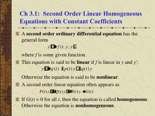
An Introduction to First-Order Linear Difference Equations With Constant Coefficients. Courtney Brown, Ph.D. Emory University. Definition of a Difference Equation. y(t+1) = ay(t) + b y(t+1) = Some constant of proportionality times y(t) plus some constant. Some interesting cases are

An Introduction to First-Order Linear Difference Equations With Constant Coefficients
E N D
Presentation Transcript
An Introduction toFirst-Order Linear Difference EquationsWith Constant Coefficients Courtney Brown, Ph.D. Emory University
Definition of a Difference Equation • y(t+1) = ay(t) + b • y(t+1) = Some constant of proportionality times y(t) plus some constant. • Some interesting cases are • y(t+1) = ay(t) … exponential growth • y(t+1) = b … a horizontal line • y(t+1) = y(t) + b … a straight sloping line
Relation to Interest • yt+1 = yt + ryt = yt(1+r) • r = rate of interest
“To Do” List for Difference Equations • Plot the equation over time • Get an analytical solution for the difference equation if it is available • Describe the model’s behavior • Determine the equilibrium values
Equilibrium Values • At equilibrium, y(t+1) = y(t) = y* • y* = ay* + b • y* - ay* = b • y*(1-a) = b • y* = b/(1-a) = the equilibrium value
Stability Criteria • y(t) will be stable if |a| < 1 • y(t) will be unstable if |a| > 1 • y(t) will oscillate if a < 0 • y(t) will change monotonically if a > 0 • y(t) will converge to a stable equilibrium value if |a| < 1
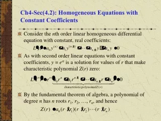
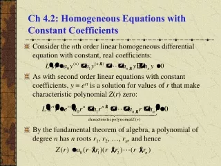
Analytic Solution: Part I • y1 = ay0 + b • y2 = ay1 + b y2 = a(ay0 + b) + b y2 = a2y0 + ab + b y2 = a2y0 + (a+1)b • y3 = ay2 + b y3 = a(a2y0 + ab + b) + b y3 = a3y0 + a2b + ab + b y3 = a3y0 + b(a2 + a + 1)
Part II: Proof by Induction Proves That • yn = any0 + b(1 + a + a2 + … + an-1), then … To find the sum 1 + a + a2 + … + an-1 write S = 1 + a + a2 + … + an-1 -aS = -(a + a2 + … + an-1 + an) S – aS = 1 – an S(1 – a) = 1 – an S = (1 – an)/(1 – a)
Part III: Thus, the solution for yn is • yn = any0 + b(1 – an)/(1 – a) or, more conveniently, • yn = b/(1-a) + [y0 – b/(1-a)]an, for a≠1 We like to write it this way because b/(1-a) is the equilibrium value, y*. If a=1, then go back to yn = any0 + b(1 + a + a2 + … + an-1) to obtain yn = y0 + b(n), the solution when a=1
Note: These solutions for the first-order linear difference equation with constant coefficients are used analytically to describe the time paths with words. Computing the time paths with a computer is done using the original equation, y(t+1) = ay(t) + b using programming loops.
a > 1, y0 > b/(1-a) Increasing, monotonic, unbounded y(t) y0 time
a > 1, y0 < b/(1-a) Decreasing, monotonic, unbounded y(t) y0 time
0 < a < 1, y0 < b/(1-a) Increasing, monotonic, bounded, convergent y(t) y* y0 time
0 < a < 1, y0 > b/(1-a) Decreasing, monotonic, bounded, convergent y(t) y0 y* time
-1 < a < 0 bounded, oscillatory, convergent y(t) y* y0 time
a < -1 unbounded, oscillatory, divergent y(t) y* y0 time
a = 1, b = 0 constant y(t) y* and y0 time
a = 1, b > 0 constant increasing y(t) y0 time
a = 1, b < 0 constant decreasing y(t) y0 time
a = -1 finite, bounded oscillatory y(t) y* y0 time
Rules of Interpretation • |a| > 1 unbounded [repelled from line b/(1-a)] • |a| < 1 bounded [attracted or convergent to [b/(1-a)] • a < 0 oscillatory • a > 0 monotonic • a = -1 bounded oscillatory All of this can be deduced from the solution yn = b/(1-a) + [y0 – b/(1-a)]an, for a≠1
Special Cases • a = 1, b = 0 constant • a = 1, b > 0 constant increasing • a = 1, b < 0 constant decreasing
Words Are Important The words used to describe the behaviors of the first-order linear difference equation with constant coefficients are used in your text. These behaviors can all be deduced from the algebra of the analytical solution to the equation.