Download
1 / 15

E N D
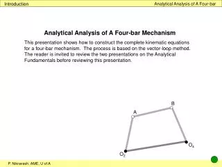
Introduction Analytical Analysis of A Four-bar Analytical Analysis of A Four-bar Mechanism This presentation shows how to construct the complete kinematic equations for a four-bar mechanism. The process is based on the vector-loop method. The reader is invited to review the two presentations on the Analytical Fundamentals before reviewing this presentation. B A O4 O2
Vector loop Analytical Analysis of A Four-bar Vector Loop for A Fourbar Define four position vectors to obtain a loop (closed chain). For notational simplification, rename the vectors. The four vectors form a vector loop equation: R2 + R3 = R1 + R4 (1) Rearranged the equation as R2 + R3 - R4 - R1 = 0 (2) Define a Cartesian x-y reference frame at a convenient position and orientation. Define angles for the vectors according to “our convention”. ► y B ► RBA R3 A 3 R4 RBO4 4 R2 RAO2 RO4O2 2 R1 O4 1 O2 x ► ► Now the vector loop equation can be transformed from vector form to algebraic form.
Algebraic Presentation of Vector Loop Analytical Analysis of A Four-bar Algebraic Form of Vector Loop Equation The vector loop equation for the fourbar in its vector form is expressed as: R2 + R3 - R4 - R1 = 0 (2) This equation is projected onto the x-axis to obtain one algebraic equation as: R2cos2 + R3cos3 - R4cos4 - R1cos1 = 0 (3-x) The projection of Eq. (2) onto the y-axis yields: R2sin2 + R3sin3 - R4sin4 - R1sin1 = 0 (3-y) ► ► y Note that the plus and minus signs in the algebraic equations (3-x) and (3-y) follow the signs in the vector loop equation (2). B R3 A 3 R4 4 R2 2 R1 O4 1 O2 x
Position Equations Analytical Analysis of A Four-bar Algebraic Form of Vector Loop Equation (cont.) The algebraic position equations for a fourbar are: R2cos2 + R3cos3 - R4cos4 - R1cos1 = 0 (3-x) R2sin2 + R3sin3 - R4sin4 - R1sin1 = 0 (3-y) These equations are called “position equations” or “position constraints”. The equations contain the following constants: R1 , R2 ,R3 ,R4 , 1 The equations contain the following variables: 2 , 3 , 4 For a specific fourbar, the constants have known (given) values. If a value is assigned to one of the variables (for example, the angle of the input link), the two equations can be solved for the other two variables. The position equations are nonlinear in the coordinates (angles).
Velocity Equations Analytical Analysis of A Four-bar Velocity Equations The algebraic position equations for a fourbar are: R2cos2 + R3cos3 - R4cos4 - R1cos1 = 0 (3-x) R2sin2 + R3sin3 - R4sin4 - R1sin1 = 0 (3-y) The time derivative of these equations yields the velocity equations or velocity constraints. Note that the variables are 2 , 3and4: - R2sin22 - R3sin33 + R4sin44 = 0 (4-x) R2cos22 + R3cos33 - R4cos44 = 0 (4-y) Where i = di/dt is the angular velocity of link i. Note that 1 = 0 since link 1 is the ground Following a position analysis, since the values of the angles are known, if a value is assigned to one of the velocities (for example, the angular velocity of the input link), the two equations can be solved for the other two angular velocities. The velocity equations are linear in the velocities, therefore easy to solve!
Acceleration Equations Analytical Analysis of A Four-bar Acceleration Equations The velocity equations for a four-bar are: - R2sin22 - R3sin33 + R4sin44 = 0 (4-x) R2cos22 + R3cos33 - R4cos44 = 0 (4-y) The time derivative of these equations yields the acceleration equations or acceleration constraints. Note that the variables are 2 , 3and4, 2, 3, and 4 : - R2sin22 - R2cos222 - R3sin33 - R3cos332 + R4sin44 + R4cos442 = 0 R2cos22 - R2sin222 + R3cos33 - R3sin332 - R4cos44 + R4sin442 = 0 Where i = di/dt is the angular acceleration of link i. These equations can be rearranged as: - R2sin22 - R3sin33 + R4sin44 = R2cos222 + R3cos332 - R4cos442 (5-x) R2cos22 + R3cos33 - R4cos44 = R2sin222 + R3sin332 - R4sin442(5-y) Note that all the quadratic velocity terms have been moved to the right hand side.
Acceleration Equations Analytical Analysis of A Four-bar Acceleration Equations (cont.) Following position and velocity analyses, since the values of the angles and angular velocities are known, if a value is assigned to one of the accelerations (for example, the angular acceleration of the input link), the two equations can be solved for the other two angular accelerations . The accelerations equations are linear in the accelerations , therefore easy to solve!
Example Analytical Analysis of A Four-bar Example Assume that for a four-bar mechanism, the following constants are given: R1 = 3.0, R2 = 1.5,R3 = 4.0,R4 = 3.5, 1 = 0.0 For the input link, link 2, know values for the angle, the angular velocity, and the angular accelerations are provided as: 2 = 60o, 2 = 1.5 rad/sec, 2 = 0.0 Determine the unknown angles, angular velocities, and angular accelerations. ► Position Analysis: The position equations from Eq. (3) are: R2cos2 + R3cos3 - R4cos4 - R1cos1 = 0 (3-x) R2sin2 + R3sin3 - R4sin4 - R1sin1 = 0 (3-y) Substituting the constant values and the value for 2in these equations yield: 1.5 cos60o + 4.0 cos3 - 3.5 cos4 - 3.0 = 0 1.5 sin60o + 4.0 sin3 - 3.5 sin4 = 0 These two nonlinear algebraic equations can be solved to determine 3and4.
Example Analytical Analysis of A Four-bar Example (cont.) How do we solve these two equations? 1.5 cos60o + 4.0 cos3 - 3.5 cos4 - 3.0 = 0 1.5 sin60o + 4.0 sin3 - 3.5 sin4 = 0 Since these are nonlinear algebraic equations, they should be solved numerically by iterative methods such as Newton-Raphson. Solution of these equations leads to two solutions. Solution 1: Solution 2: 3 = 29.7o 4 = 69.5o ► 3 = 270.3o 4 = 230.5o ►
Example Analytical Analysis of A Four-bar Example (cont.) Velocity Analysis: The velocity equations from Eq. (4) are: - R2sin2 2 - R3sin3 3 + R4sin4 4 = 0 (4-x) R2cos2 2 + R3cos3 3 - R4cos4 4 = 0 (4-y) Substituting the constant quantities yields: -1.5 sin2 2 - 4.0 sin3 3 + 3.5 sin4 4 = 0 1.5 cos2 2 + 4.0 cos3 3 - 3.5 cos4 4 = 0 The given values for the angle and the angular velocity of the input link are 2 = 60oand2 = 1.5 rad/sec. Substituting these values yields -1.5 sin 60o(1.5) - 4.0 sin3 3 + 3.5 sin4 4 = 0 1.5 cos 60o(1.5) + 4.0 cos3 3 - 3.5 cos4 4 = 0 The values of 3 and 4 are also known, but we must decide which configuration we want to consider!
Example Analytical Analysis of A Four-bar Example (cont.) Velocity Analysis: Solution 1: For 3 = 29.7oand 4 = 69.5o, the velocity equations become: -1.5 sin60o(1.5) - 4.0 sin29.7o3 + 3.5 sin69.5o4 = 0 1.5 (cos60o(1.5) + 4.0 cos29.7o3 - 3.5 cos69.5o4 = 0 Or, -1.983 + 3.284 = 1.95 3.483 - 1.234 = -1.13 Solving these equations provide values for the unknown angular velocities: 3 = -0.15 4 = 0.51
Example Analytical Analysis of A Four-bar Example (cont.) Velocity Analysis: Solution 2: For 3 = 270.3oand 4 = 230.5o, the velocity equations become: -1.5 sin60o (1.5) - 4.0 sin270.3o3 + 3.5 sin230.5o4 = 0 1.5 cos60o (1.5) + 4.0 cos270.3o3 - 3.5 cos230.5o4 = 0 Or, 4.003 - 2.704 = 1.95 0.023 + 2.234 = -1.13 Solving these equations provide values for the unknown angular velocities: 3 = 0.15 4 = -0.51
Example Analytical Analysis of A Four-bar Example (cont.) Acceleration Analysis: The acceleration equations from Eq. (5) are: - R2sin22 - R3sin33 + R4sin44 = R2cos222 + R3cos332 - R4cos442 (5-x) R2cos22 + R3cos33 - R4cos44 = R2sin222 + R3sin332 - R4sin442(5-y) Substituting the constant quantities, the given values for the input link; i.e., 2 = 60o, and2 = 1.5 rad/sec, and 2 = 0 yields - 1.5 sin60o(0)- 4.0 sin3 3 + 3.5 sin4 4 = 1.5 cos60o(1.5)2 + 4.0.cos3 32 - 3.5 cos4 42 1.5 cos60o(0)+ 4.0 cos3 3 - 3.5 cos4 4 = 1.5 sin60o(1.5)2 + 4.0 sin3 32 - 3.5 sin4 42 The values of 3 and 4 are also known, but we must decide which configuration we want to consider!
Example Analytical Analysis of A Four-bar Example (cont.) Acceleration Analysis: Solution 1: For 3 = 29.7o, 4 = 69.5o, 3 = -0.15 , and 4 = 0.51, the acceleration equations become: - 1.5 sin60o(0) - 4.0 sin29.7o3 + 3.5 sin69.5o4 = 1.5 cos60o(1.5)2 + 4.0.cos29.7o-0.15 2 - 3.5 cos69.5o(0.51)2 1.5 cos60o(0) + 4.0 cos29.7o3 - 3.5 cos69.5o4 = 1.5 sin60o(1.5)2 + 4.0 sin29.7o-0.15 2 - 3.5 sin69.5o(0.51)2 Or, -1.983 + 3.284 = 1.45 3.483 - 1.234 = 2.12 Solving these equations provide values for the unknown angular accelerations: 3 = 0.97 4 = 1.03
Example Analytical Analysis of A Four-bar Example (cont.) Acceleration Analysis: Solution 2: For 3 = 270.3o,4 = 230.5o, 3 = 0.15 , and 4 = -0.51, the acceleration equations become: - 1.5 sin60o(1) - 4.0 sin270.3o3 + 3.5 sin230.5o4 = 1.5 cos60o(1.5)2 + 4.0.cos270.3o0.15 2 - 3.5 cos620.5o(-0.51)2 1.5 cos60o(1) + 4.0 cos270.3o3 - 3.5 cos230.5o4 = 1.5 sin60o(1.5)2 + 4.0 sin270.3o0.15 2 - 3.5 sin630.5o(-0.51)2 Or, 4.003 - 2.704 = 2.26 0.023 + 2.234 = 3.53 Solving these equations provide values for the unknown angular accelerations: 3 = 1.62 4 = 1.57


