Visual Resource Inventory
Visual Resource Inventory. Comparison of Geodatabase to BLM Manual H-8410: Field Sheets Version 1.1 Draft March 2011. Bureau of Land Management – Visual Resource Management System.

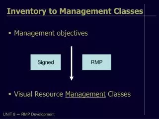
Visual Resource Inventory
E N D
Presentation Transcript
Visual Resource Inventory Comparison of Geodatabase to BLM Manual H-8410: Field Sheets Version 1.1 Draft March 2011
Bureau of Land Management – Visual Resource Management System • BLM’s VRM system provides a way to identify and evaluate scenic values to determine the appropriate levels of management. It also provides a way to analyze potential visual impacts and apply visual design techniques to ensure that surface-disturbing activities are in harmony with their surroundings. • The BLM VRM system consists of two stages: • Inventory (Visual Resource Inventory) • Analysis (Visual Resource Contrast Rating) • The inventory stage involves identifying the visual resources of an area and assigning them to inventory classes using BLM’s visual resource inventory process. The process involves rating the visual appeal of a tract of land, measuring public concern for scenic quality, and determining whether the tract of land is visible from travel routes or observation points. (Excerpted from Web Site) The Bureau has developed a Data Standard that pertains to Visual Resource Inventories. This Data Standard has been physically implemented within a geographic information system (GIS) as an ESRI Geodatabase; which is detailed in the Implementation Guidelines. This document serves to provide an aid in documenting the inventory within the GIS environment, and provides information on cross-walking the information from the field inventory sheets to the Geodatabase. This document does not replace BLM Manual 8410.
Scenic Quality Evaluation • (Excerpts from Manual H-8410-1 - Visual Resource Inventory) Scenic quality is a measure of the visual appeal of a tract of land. In the visual resource inventory process, public lands are give an A, B, or C rating based on the apparent scenic quality which is determined using seven key factors: landform, vegetation, water, color, adjacent scenery, scarcity, and cultural modifications. Delineating Scenic Quality Rating Units (SQRU's). The planning area is subdivided into scenic quality rating units for rating purposes. Rating areas are delineated on a basis of: like physiographic characteristics; similar visual patterns, texture, color, variety, etc.; and areas which have similar impacts from man-made modifications. Evaluating Scenic Quality. Evaluate each SQRU by observing the area from several important viewpoints. Scores should reflect the overall impression of the area. After evaluating all the SQRU's, show the scenic ratings on the scenic quality overlay (see Illustration 7). Record the rating on the Scenic Quality Rating Summary - Bureau Form 8400-5 (see Illustration 4). Bureau Form 8400-1 (see Illustration 3) may be used as a worksheet for completing each scenic quality evaluation. A photographic record should be maintained for the area. Photographs and completed evaluation forms should be filed for future reference. Scenic Quality Rating Units and Inventory Observation Points shall be represented as geometric features in the GIS, with the related GIS tables being used to document the scores and associated information for each SQRU and IOP. Refer to BLM Manual 8410 for instructions on conducting a visual resource inventory.
Scenic Quality Evaluation – Example Field Sheet and Summary Sheet Form 8400-1 Information from these sheets are recorded in the GIS vri_sqru_poly feature class, and the related tables (vri_sqru_factors_tbl and vri_sqru_landscape_tbl) 08/15/1985 08/16/1985 Green River Green River Moab Moab 024 Bob Tumwater, Russ Grimes, Pete Jordon Bob Tumwater, Russ Grimes, Pete Jordon Form 8400-5 Deeply cut side canyons with vertical walls leading into flat open valley w/ slow meandering river Simple forms created by patterns in vegetation Oval, elongated, and linear Colorful waterway Rolling hills, colorless, little veg Flat, colorless, barren Water, scenic cliffs, interesting veg Scenic cliffs Flat, colorless, barren Water, riverside veg, colorful cliffs Good mixture of color, topo & veg Rugged but otherwise mountainous Mountainous with good view of N.P. 2 2 2 1 3 2 2 3 2 2 5 0 0 4 0 0 5 0 0 0 0 0 0 0 0 0 0 0 0 0 4 2 2 4 4 2 4 3 2 2 001 002 003 004 005 006 007 008 009 010 3 3 2 4 4 1 4 3 3 1 4 1 1 3 3 1 4 3 2 2 2 3 3 3 4 2 3 3 2 3 20 11 10 19 18 8 22 15 11 10 A C C A B C A B C C Horizontal and vertical in cliff formations, jagged ridge lines, and meandering river Irregular, indistinct Rounded, vertical Orange and greys dominant, deep blue in settling pond Dark green in river bottom, grey elsewhere Light green and grey Coarse Medium grain, sparse, and uneven random Uneven This SQRU includes the flat and meandering river bed of the Colorado River and the deeply dissected canyons to the north. It differs in landform and vegetation from the surrounding areas. The rock formations and topography are fairly common in the physiographic province but it is uncommon to have a river flowing through this type of landscape. The potash plant which lies in the middle of this area is a major visual intrusion which can be seen from several outlooks and the river. Comments on 4e – Adjacent scenery: The high scenic rating of “4” was given to this factor because of the high scenic value of the surrounding areas that can be seen from within the SQRU. These scenic areas include Behind-the-Rocks area, Canyonlands country, and the La Sal mountains. 4 2 See explanation above 4 -3 18 5 (-3) 20
That Portion of the Geodatabase that Applies to Scenic Quality Rating Units and Inventory Observation Points FEATURE CLASSESRELATED TABLES GUIDANCE TABLES Inventory Observation Points Scenic Quality Rating Unit: Landscape Character and Element Table Scenic Quality Rating Unit Polygons (each polygon corresponds to a scenic quality rating unit area, and may be a multi-part feature) Polygon Arcs (defines polygon boundaries and documents feature level metadata) Scenic Quality Rating Unit: Scenic Factor Scores Table Inventory Observation Point to Associated Scenic Quality Rating Unit Polygon Table (each record in the table is related to each feature class through a one-to-many relationship class)
Inventory Observation Points GIS Feature Class, Table and Attributes An Inventory Observation Point (IOP) is either an important viewpoint or is representative of the scenic quality rating unit being evaluated for scenic quality. Each SQRU will have at least one Inventory Observation Point. Each IOP may be used to evaluate one or more scenic quality rating units. Within the geodatabase, IOPs are only associated with SQRUs. Feature class: vri_iop_pt Information about the inventory observation point is recorded for each point in the feature class Attributes: IOP_ID ADMIN_ST ADM_OFC_CD ADM_UNIT_CD IOP_NR IOP_NAME ELEV_FT IOP_RPRSNT IOP_MTHD IOP_CMMNTS CREATE_DATE CREATE_BY MODIFY_DT MODIFY_BY PT_SRC_TYPE PT_SRC_DESC ACCURACY_FT GlobalID Table: vri_iop_sqru_tbl Information about each observation point and scenic quality rating unit pair is recorded in the table Attributes: IOP_ID SQRU_ID OBSRVR_FT DT_ANLZ TM24_ANLZ EVALUATORS GlobalID
Scenic Quality Rating Units GIS Feature Class, Tables and Attributes Feature class: vri_sqru_poly The scenic quality total score and code is recorded for each polygon in the scenic quality rating unit feature class Attributes: SQRU_ID ADMIN_ST ADM_OFC_CD ADM_UNIT_CD SQRU_NR SQRU_NAME ADMIN_FO_NAME SQRU_EVAL SQRU_ORIG_DT SQRU_MOD_DT SQ_TOT_SCR SQ_CODE SQ_CODE_TX SQRU_NRTV1 & 2 SQ_ANLZ_MTHD GlobalID Table: vri_sqru_factors_tbl The scores and explanatory text for the individual factors of scenic quality are recorded in the factors table Attributes: SQRU_ID SQ_LFORM_SCR SQ_VEG_SCR SQ_WATER_SCR SQ_COLOR_SCR SQ_ADJCNT_SCR SQ_SCARC_SCR SQ_CULT_SCR SQ_LFORM_TX SQ_VEG_TX SQ_WATER_TX SQ_COLOR_TX SQ_ADJCNT_TX SQ_SCARC_TX SQ_CULT_TX GlobalID Table: vri_sqru_landscape_tbl The descriptions of the different elements for landscape character are recorded in the landscape table Attributes: SQRU_ID LFORM_FORM LFORM_LINE LFORM_COLOR LFORM_TEXTURE VEG_FORM VEG_LINE VEG_COLOR VEG_TEXTURE STRUCT_FORM STRUCT_LINE STRUCT_COLOR STRUCT_TEXTURE GlobalID
Cross-Walk Scenic Quality Field Sheet to GIS Feature Class & Tables Scenic Quality Field Inventory Sheet GIS Elements & Attributes Form 8400-1 The GIS attributes are color coded according to the feature class or table: SQRU_ORIG_DT ADM_UNIT_CD ADMIN_FO_NAME FC vri_sqru_poly TBL vri_sqru_factors_tbl TBL vri_sqru_landscape_tbl SQRU_NR SQRU_EVAL LFORM_FORM VEG_FORM STRUCT_FORM • This implementation contains the following new attributes: • SQ_ANLZ_MTHD • information on how the scenic quality was conducted from the different IOP’s for the rating unit. • SQ_CODE_TX • information explaining the assigned code • All records for each scenic quality rating unit (polygon) are linked to each other through a primary key: • SQRU_ID • Concatenated value based on the prefix “SQ” + administrative unit code (ADM_UNIT_CD) + scenic quality rating unit number (SQRU_NR) LFORM_LINE VEG_LINE STRUCT_LINE VEG_COLOR STRUCT_COLOR LFORM_COLOR LFORM_TEXTURE VEG_TEXTURE STRUCT_TEXTURE SQRU_NRTV1 and SQRU_NRTV2 (if needed for overflow text) SQ_LFORM_SCR SQ_VEG_SCR SQ_WATER_SCR SQ_COLOR_SCR SQ_ADJCNT_SCR SQ_SCARC_SCR SQ_CULT_SCR The value for each attribute corresponds to a score below SQ_LFORM_TX SQ_VEG_TX SQ_WATER_TX SQ_CODE SQ_COLOR_TX SQ_ADJNT_TX SQ_SCARC_TX SQ_CULT_TX SQ_TOT_SCR
GIS Feature Classes : Scenic Quality & Inventory Observation Points Example of the feature classes and attribute tables for the Inventory Observation Points and Scenic Quality Rating Units. Each feature has a unique identifier which is used as a primary key. Each IOP is related to one or more SQRU Each SQRU is related to one or more IOP
GIS Related Tables: Scenic Quality & Inventory Observation Points vri_iop_pt: IOP_ID (IOP Unique ID) is primary key Related table to show the IOP to SQRU pairs vri_sqru_poly: SQRU_ID (SQRU Unique ID) is Primary Key Related tables to record the Scores for the seven factors of scenic quality, and the landscape characteristics
Sensitivity Level Analysis • (Excerpts from Manual H-8410-1 - Visual Resource Inventory) Sensitivity levels are a measure of public concern for scenic quality. Public lands are assigned high, medium, or low sensitivity levels by analyzing the various indicators of public concern. Delineation of Sensitivity Level Rating Units (SLRU's). There is no standard procedure for delineating SLRU's. The boundaries will depend on the factor that is driving the sensitivity consideration. Documenting Sensitivity Level. For each rating unit, analyze and rate the sensitivity level (as low, moderate, or high) for each of the following factors: Type of Users, Amount of Use, Public Interest, Adjacent Land Uses, Special Areas, and Other Factors. Determine the overall sensitivity level for each rating unit. This is a process which requires careful analysis of all the factors. Prepare a summary statement with the essential facts and rationale to support the conclusions reached on sensitivity levels. At a minimum, the summary data must be entered on Form 8400-6 (see Illustration 8). Backup information used to evaluate each of the factors should be maintained with the inventory record. Prepare an overlay (see Illustration 9) showing the sensitivity rating units and ratings Sensitivity Level Rating Units shall be represented as geometric features in the GIS, with the related GIS table being used to document the rating for each sensitivity level factor and its associated explanation. Refer to BLM Manual 8410 for instructions on conducting a visual resource inventory.
Sensitivity Level Analysis – Example Summary Sheet Form 8400-6 08/15/1985 Information from this sheet are recorded in the GIS vri_slru_poly feature class, and the related table (vri_slru_ratings_tbl) Green River Moab Bob Tumwater, Russ Grimes, Pete Jordon 001 H HHHH - H within f/m zone of I-70 & U163 002 H L M L H - H visible from river and floatboat users 003 L LLLL - L isolated area with low scenic values 004 H M H M M - H f/m zone for state park entrance road
Section of the Geodatabase that Applies to Sensitivity Level Rating Units FEATURE CLASSESRELATED TABLE GUIDANCE TABLES Sensitivity Level Rating Units GIS Feature Class, Table and Attributes Feature class: vri_slru_poly The sensitivity level overall rating is recorded for each polygon in the sensitivity level rating unit feature class. Each polygon represents one sensitivity level rating unit, and may be a multi-part feature Attributes: Table:vri_slru_ratings_tbl The ratings and explanatory text for the individual factors for sensitivity are recorded in the ratings table Attributes: SLRU_ID SL_USERS_RT SL_USERS_TX SL_AREAUSE_RT SL_AREAUSE_TX SL_PUBLIC_RT SL_PUBLIC_TX SL_ADJNT_RT SL_ADJNT_TX SL_SPCL_RT SL_SPCL_TX SL_OTHR_RT SL_OTHR_TX GlobalID SLRU_ID ADMIN_ST ADM_OFC_CD ADM_UNIT_CD SLRU_NR ADMIN_FO_NAME SLRU_EVAL SLRU_ORIG_DT SLRU_MOD_DT SL_ORVL_RT SL_ORVL_TX SLRU_NRTV GlobalID
Cross-Walk Sensitivity Level Summary Sheet to GIS Feature Class & Table Sensitivity Level Rating Sheet GIS Elements & Attributes Form 8400-6 SLRU_ORIG_DT The GIS attributes are color coded according to the feature class or table: ADM_UNIT_CD ADMIN_FO_NAME SLRU_EVAL FC vri_slru_poly TBL vri_slru_ratings_tbl SLRU_NR SL_ORVL_RT SL_ORVL_TX • This implementation contains the following new attributes: • SLRU_NRTV • Descriptive information about the SLRU as it relates to sensitivity, as well as any additional information on how the area for the SLRU area was determined. • All records for each sensitivity level rating unit (polygon) are linked to each other through a primary key: • SLRU_ID • Concatenated value based on the prefix “SL” + administrative unit code (ADM_UNIT_CD) + sensitivity level rating unit number (SLRU_NR) SL_OTHR_RT and SL_OTHR_TX SL_SPCL_RT and SL_SPCL_TX SL_ADJNT_RT and SL_ADJNT_TX SL_PUBLIC_RT and SL_PUBLIC_TX SL_AREAUSE_RT and SL_AREAUSE_TX SL_USERS_RT and SL_USERS_TX Note: The attribute pairs, above, are for recording the rating and explanation for each of the sensitivity level factors
GIS Feature Class & Tables: Sensitivity Level Attribute Values Example of the feature class, attribute table and related table for the Sensitivity Level Rating Units. Each feature has a unique identifier which is used as a primary key. Each polygon in the feature class should have a matching record in the related table.
Distance Zones • (Excerpts from Manual H-8410-1 - Visual Resource Inventory) Landscapes are subdivided into 3 distanced zones based on relative visibility from travel routes or observation points. The foreground-middleground (fm) zone includes areas seen from highways, rivers, or other viewing locations which are less than 3 to 5 miles away. Seen areas beyond the foreground-middleground zone but usually less than 15 miles away are in the background (bg) zone. Areas not seen as foreground-middleground or background (i.e., hidden from view) are in the seldom-seen (ss) zone. Mapping Distance Zones. Prepare a distance zone overlay (see Illustration 10). Distance zones should be mapped for all areas. While they are not necessary to determine classes… distance zones can provide valuable data during the RMP process when adjustments to VRM classes are made to resolve resource allocation conflicts. Coordinating Distance Zones Delineation and Sensitivity Level Analyses. It is recommended that distance zones be delineated before the sensitivity analysis is done. The distance zone delineations provide valuable information that can be very useful in the sensitivity analysis. For example, the foreground-middleground zones are more visible to the public and changes are more noticeable and are more likely to trigger public concern. Also, the boundaries of the distance zones are very useful in helping to establish sensitivity rating units. Distance Zones shall be represented as geometric features in the GIS. The methodology used to determine the visual distance zone represented by the polygon will be documented (i.e. raster based viewshed analysis, GIS buffer operation, or field observation). Additionally, this implementation allows for the near-foreground distance zone (up to ¼ mile) that is to be used only when inventorying a National Scenic or Historic Trail.
Distance Zones – Example of Distance Zone Overlay Illustration 10 - Distance Zone Overlay Big Flat Squaw Park - West Planning Unit - Bureau of Land Management
Section of the Geodatabase that Applies to Visual Distance Zones FEATURE CLASSESRELATED TABLE GUIDANCE TABLES Visual Distance Zones GIS Feature Class Feature class: vri_vdz_poly The visual distance zone classification is recorded for each polygon in the visual distance zone feature class Attributes: • This implementation contains the following: • VDZ_NRTV • Descriptive information about the VDZ as it relates to visibility. Comments could include information about the natural or built environment that affects the distance zone, any visual obstructions, or other conditions. • VDZ_MTHD • Methodology used to determine the visual distance zone presented by the polygon. Examples could include: GIS buffer analysis of roadway, field observation, GIS buffer operation followed by field observation and adjustments, viewshed analysis using DEM/TIN, previously defined distance zones, manual delineation of distance zones and viewsheds, etc. • Each visual distance zone polygon has a Unique Identifier (primary key): • VDZ_ID • Concatenated value based on the prefix “DZ” + administrative unit code (ADM_UNIT_CD) + visual distance zone number (VDZ_NR) VDZ_ID ADMIN_ST ADM_OFC_CD ADM_UNIT_CD VDZ_NR ADMIN_FO_NAME SLRU_EVAL SLRU_ORIG_DT SLRU_MOD_DT VDZ_CODE VDZ_MTHD VDZ_NRTV GlobalID
GIS Feature Class & Tables: Distance Zones Example of the feature class and attribute table for Visual Distance Zones. The presence of cities and towns, and transportation features such as roads and trails, make all areas shown fall within the foreground-middleground zone for visual distance. There is no related table for Visual Distance Zones. The Near-Foreground zone is to be used only when conducting an inventory for a National Scenic and Historic Trail.
Visual Resource Inventory Classes • (Excerpts from Manual H-8410-1 - Visual Resource Inventory) Purposes of Visual Resource Classes. Visual resource classes are categories assigned to public lands which serves two purposes: (1) an inventory tool that portrays the relative value of the visual resources, and (2) a management tool that portrays the visual management objectives. There are four classes (I, II, III, and IV). Visual Resource Inventory Classes. Visual resource inventory classes are assigned through the inventory process. This is accomplished by combining the 3 overlays for scenic quality, sensitivity levels, and distance zones and using the guidelines shown in the matrix (see Illustration 11) to assign the proper class. The end product is a visual resource inventory class overlay (see Illustration 12). Inventory classes are informational in nature and provide the basis for considering visual values in the RMP process. They do not establish management direction and should not be used as a basis for constraining or limiting surface disturbing activities. Rehabilitation Areas. Areas in need of rehabilitation from a visual standpoint should be flagged during the inventory process. The level of rehabilitation will be determined through the RMP process by assigning the VRM class approved for that particular area. Visual Resource Inventory Classes shall be represented as geometric features in the GIS. These features shall be derived from the feature classes for scenic quality, sensitivity levels, and distance zones.
Determining Visual Resource Inventory Classes Basis for Determining Visual Resource Inventory Classes Class I. Class I is assigned to all special areas where the current management situations requires maintaining a natural environment essentially unaltered by man. Classes II, III, and IV. These classes are assigned based on combinations of scenic quality, sensitivity levels, and distance zones. * If adjacent area is Class III or lower assign Class III, if higher assign Class IV
Section of the Geodatabase that Applies to Visual Resource Inventory Classes FEATURE CLASSESRELATED TABLE GUIDANCE TABLES Visual Resource Inventory Classes GIS Feature Class Feature class: vri_class_poly The polygons and associated inventory classes for this feature class are derived from the other feature classes for scenic quality, sensitivity and distance. Attributes: • This implementation contains the following: • VRI_CLASS_TX • Optional text explaining why a specific visual resource inventory class was assigned. • VRI_REHAB_IND • Yes/No value indicating that the area was identified as needing rehabilitation during the visual resource inventory . • VRI_SPCL_IND • Yes/No value indicating that the area was identified as possessing unique landscape and/or visual quality characteristics during the visual resource inventory . • Each visual resource inventory class polygon has a Unique Identifier (primary key): • VRI_AREA_ID • Concatenated value based on the prefix “VRI” + administrative unit code (ADM_UNIT_CD) + VRI area number (VRI_AREA_NR) VRI_AREA_ID ADMIN_ST ADM_OFC_CD ADM_UNIT_CD VRI_AREA_NR ADMIN_FO_NAME VRI_EVAL VRI_ORIG_DT VRI_MOD_DT VRI_CLASS_CODE VRI_CLASS_TX BLM_ACRE SQ_CODE SL_OVRL_RT VDZ_CODE VRI_REHAB_IND VRI_SPCL_IND GlobalID
GIS Feature Class & Tables: Visual Resource Inventory Classes Example of the feature class and attribute table for the final Visual Resource Inventory Classes. The polygons depicting the inventory classes are derived through a process where the scenic quality, visual sensitivity and distance zones are combined. The Visual Resource Inventory Classes are informational in nature, and do not constitute a management class. However, they do serve as a baseline of information from which the affected environment sections of all subsequent NEPA analysis should reference.
Deriving VRI Classes: Example Using Union, Dissolve & Eliminate Tools Sensitivity • What follows demonstrates only one example of how the final inventory class polygons may be derived. Regardless of methodology, the process should be documented with any interim products maintained. • Example using the Union Tool • The Union tool is accessed in Arc Toolbox > Analysis Tools > Overlay • The union will be performed between SLRU, SQRU and VDZ feature classes with output to an interim file Scenic Quality ArcTools Union Tool
Deriving VRI Classes: Example Using Union, Dissolve & Eliminate Tools VRI_Union feature class is output of union • Output of the Union Tool • Geoprocessing results were written to an interim feature class (VRI_Union) • All attributes from the three inputs are captured in the output • Input polygons are “cracked” and then reassembled so that each new polygon has a unique boundary and SQ, SL and DZ combination that corresponds to the different polygons of the inputs • The dissolve tool may then be used to combine adjacent union output polygons that have the same SQ, SL and DZ value Only the attributes of interest are shown at right
Deriving VRI Classes: Example Using Union, Dissolve & Eliminate Tools VRI_Union (input for dissolve) • The Dissolve Tool • The Dissolve Tool is accessed in Arc Toolbox > Data Management Tools > Generalization • The dissolve will be performed against the VRI_Union interim feature class • Geoprocessing results were written to an interim feature class (VRI_Union_Dissolve) • The SQ_CODE, SL_OVRL_RT, and VDZ_CODE attributes are used in performing the dissolve. There will be no statistics, and single-part (not multi-part) polygons will be created. Dissolve Tool aggregates features based on specific attributes ArcTools Dissolve Tool
Deriving VRI Classes: Example Using Union, Dissolve & Eliminate Tools VRI_Union_Dissolve feature class is output of dissolve • Output of the Dissolve Tool • Geoprocessing results were written to an interim feature class (VRI_Union_Dissolve) • The SQ_CODE, VDZ_CODE and SL_OVRL_RT attributes are captured in the output • Input polygons are aggregated so that adjacent polygons with the same value for SQ, SL and DZ are combined • This tool will reduce the number of polygons, but there may still may a large number of very small polygons • The small polygons may then be “appended” onto an adjacent larger polygon using the eliminate tool
Deriving VRI Classes: Example Using Union, Dissolve & Eliminate Tools VRI_Union_Dissolve (input for eliminate) • The EliminateTool • The EliminateTool is accessed in Arc Toolbox > Data Management Tools > Generalization • The eliminate will be performed against selected features (in this case, acres < 50) found within the VRI_Union_Dissolve interim feature class • Geoprocessing results are written to an interim feature class (VRI_Union_Dissolve_ElimLT50Acre) Selected features are shown above in cyan – these features are less than 50 acres in size, and will be merged into an adjacent polygon. BEFORE ELIMINATE AFTER ELIMINATE
Deriving VRI Classes: Example Using Union, Dissolve & Eliminate Tools • Output of the Process • Geoprocessing results were written to an interim feature class (VRI_Union_Dissolve_ElimLT50Acre) • All attributes from the three inputs are captured in the output • Load the interim data into the vri_class_poly feature class