Correlation and Regression

1. Correlation and Regression

2. Correlation. • ‘Correlation’ is a statistical tool which measure the strength of linear relationship between two variables. • It can not measure strong non-linear relationship. • It can not measure Cause and Effect. • “Two variables are said to be in correlated if the change in one of the variables results in a change in the other variable”. • Types of Correlation • There are two important types of correlation. • (1) Positive and Negative correlation and • (2) Linear and Non – Linear correlation.

3. Positive and Negative Correlation • If the values of the two variables deviate in the same direction i.e. if an increase (or decrease) in the values of one variable results, on an average, in a corresponding increase (or decrease) in the values of the other variable the correlation is said to be positive. • Some examples of series of positive correlation are: • Heights and weights; • Household income and expenditure; • Price and supply of commodities; • Amount of rainfall and yield of crops. • Correlation between two variables is said to be negative or inverse if variables deviate in opposite direction • Some examples of series of negative correlation are: • Volume and pressure of perfect gas; • Current and resistance [keeping the voltage constant] . • Price and demand of goods etc.

4. The Coefficient of Correlation • It is denoted by ‘r’ which measures the degree of association between the values of related variables given in the data set. • -1≤ r ≤1 • If r >0 variables are said to be positively correlated. • If r<0 variables are said to be negatively correlated. • For any data set if r = +1, they are said to be perfectly correlated positively • if r = -1 they are said to be perfectly correlated negatively, and • if r = 0 they are uncorrelated.

6. Correlation In Statistica. • Got to “Statistic” tab and “Basic statistic”. • Click “Correlation matrix” tab click ok. • If you want to get correlation only on two variables, go to the “Two variable list” and select those two variables which are required. • Click ok and then click on summary.

7. If you want to get the correlation matrix for all variables, go to “Two variable list” tab and click on “select all” tab, click ok. • Click the summary , you will get correlation matrix.

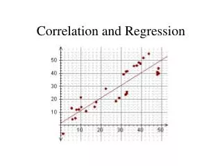
8. To get scatter plot – click on “Scatter plot of variables” and then select the variables and click ok. • You will get the scatter plot as it has came in the right side.

9. To get another kind of Scatter plot click on “Graphs” option. • You will get a series of scatter plot for each and every pairs of variable. • The second plot is showing one of those.

10. Regression • Regression analysis, in general sense, means the estimation or prediction of the unknown value of one variable from the known value of the other variable. • If two variables are significantly correlated, and if there is some theoretical basis for doing so, it is possible to predict values of one variable from the other. This observation leads to a very important concept known as ‘Regression Analysis’. • It is specially used in business and economics to study the relationship between two or more variables that are related causally and for the estimation of demand and supply graphs, cost functions, production and consumption functions and so on.

11. Thus, the general purpose of multiple regression is to learn more about the relationship between several independent or predictor variables and a dependent or output variable. • Suppose that the Yield in a chemical process depends on Temperature and the Catalyst concentration, a multiple regression that describe this relationship is, Y=b0+b1*X1+b2*X2+€ → (a) Where Y = Yield. X1 = Temp:, X2 = Catalyst cont:. This is multiple linear regression model with 2 regressors. • The term linear is used because equation (a) is a linear function of the unknown parameters bi’s.

12. Regression Models. • Depending on nature of relationship regression models are two types. • Linear regression model, including • Simple-linear regression (one indep: var.) • Multiple-linear regression. • Non-Linear regression model, including • Polynomial regression. • Exponential regression ,etc.

13. Assumption of Linear regression model. • The relationship between Y (dependent variable) and independent variables are linear. • The independent variables are mutually independent to each other. • The errors are uncorrelated to each other. • The error term has fixed variance. • The errors are Normally distributed.

14. Data set and Objective. • The current data set has been taken from a chemical process where we have two input or independent parameters , Temperature and Catalyst feed rate Response or output parameter : Viscosity of the yield. • Objective. • Establish the linear relation of dependent variable with independent variables. • Estimate regression coefficients to find out which variable has significant effect on the response variable. • Check the model adequacy with the help of assumptions.

15. Data set.

16. Assumption of Linearity. • First of all, as is evident in the name multiple linear regression, it is assumed that the relationship between variables is linear. • In practice this assumption can virtually never be confirmed; fortunately, multiple regression procedures are not greatly affected by minor deviations from this assumption. • However, as a rule it is prudent to always look at bivariate scatter plot of the variables of interest. • If curvature in the relationships is evident, one may consider either transforming the variables, or explicitly allowing for nonlinear components.

17. Scatter plot. • Go to “Graph” option and select “Scatter plot”. • Click on “variable” tab and select the variables in the above way. • Click ok and select the option “Multiple” and “Confidence” . This will help you to plot multiple graph in a single window. (If you have large number of variables then plot it separately)

18. The scatter plot has established linear relationship of the dependent with independent variables. • Here Viscosity and Temp are linearly related to each other, but Viscosity and Catalyst concentration are not.

19. Parameter Estimation. • The regression coefficient  (beta) is the average amount of change in the dependent (either in positive or negative direction, depending on the sign of ’s) when the independent changes one unit and other independents are held constant. • The b coefficient is the slope of the regression line. • Intercept (constant,α)- It is the value of dependent variable when all indep: are set to zero. • For any independent variable if the corresponding >0, then that variable is positively correlated with dependent variable, negatively otherwise. • OLS (ordinary least squares) is used to estimate the coefficients in such a way that the sum of the squared deviations of the distances of all the points to the line is minimized.

20. The confidence interval of the regression coefficient. We can 95% confident that the real regression coefficient for the population lies within this intervals. • If the confidence interval includes 0, then there is no significant linear relationship between x and y. • The confidence interval of y – It indicates 95 times out of a hundred, the true mean of y will be within the confidence limits around the observed mean of n sampled. • SEE (Standard error of estimate) is the standard deviation of the residuals. In a good model, SEE will be markedly less than the standard deviation of the dependent variable. • It can be used to compare the accuracy of different models, lesser the value better the model.

21. F-test and P-value: Testing the Overall Significance of the Multiple Regression Model. • It assume the null hypothesis, H0: b1 = b2 = ... = bk = 0 H1: At least one bi does not equal 0. • If H0 is rejected (if p<.05) we can conclude that, • At least one bi differs from zero. • The regression equation does a better job of predicting the actual values of y. • t-test:Testing the Significance of a Single Regression Coefficient. • Is the independent variable xi useful in predicting the actual values of y ? For the Individual t-test H0: bi = 0 H1: bi ≠0 • If H0 is rejected (if p<.05) The related X has a significant contribution on the dependent variable,

22. R^2 (coefficient of determination)-Is the percent of the variance in the dependent explained uniquely or jointly by the independents. • R-squared can also be interpreted as the proportionate reduction in error in estimating the dependent when knowing the independents. • Adjusted R-Square It is an adjustment of R-square when one has a large number of independents • It is possible that R-square will become artificially high simply because some independent variable "explain" small parts of the variance of the dependent. • If there is a huge difference between R-square and Adjusted R-square then we can assume that some unimportant independent variables are present in the data set. • If inclusion of a variable reduces Adjusted R-square it will be identified as a nonsense parameter for the model.

23. Estimating coefficients. • Go to “Statistics” tab and select “Multiple Regression”. • Select the variables and click ok again click ok. • Now click “Summary regression results”.

24. Left side table showing the model accuracy. • R-square- Describing the amount of variability that has been explained by indep: variables, here it is approx. 93%. • Adjusted R-square – Give an indication whether there is any insignificant factor or not. • Adj: R square should be close to Multiple R square, if it is very smaller than R square then we should go for stepwise regression. (Adjusted R square always < or = Multiple R square.)

25. Interpretation of Result. • Here R square and Adjusted R square are very close to each other, which indicate a good model. • In regression analysis R square value will always increase with the inclusion of parameters , but Adjusted R square may not be, this indicate the presence of nuisance parameters in the model. • The p value for F test is significant (left table) indicate, there is at least one variable which has significant contribution to the model. • The p values for t-test are all significant (as p<.05)(2nd table) which indicate all these variables has significant effect on the response.

26. Multicollinearity. • Definition Multicollinearity refers to excessive correlation of the independent variables. • Ideally independent variable should be uncorrelated to each other (according to the assumption). • If the correlation is excessive (some use the rule of thumb of r >0.90), standard errors of the beta coefficients become large, making it difficult or impossible to assess the relative importance of the predictor variables. • But multicollinearity does not violate OLS assumption, it still gives unbiased estimate of the coefficient.

27. Detecting Multicollinearity • ToleranceThe regression of any independent variable on all the other independents, ignoring the dependent. As a rule of thumb, if Tolerance ≤ 0.10, a problem with multicollinearity is indicated. • VIF (Variance-inflation factor) Is simply the reciprocal of tolerance. As a rule thumb, if VIF > 10 , a problem with multicollinearity is indicated. • C.I (condition indices) Another index for checking multicollinearity. As rule thumb , if C.I >30 serious multicollinearity is present in the data set.

28. Some other indication of multicollinearity. • If none of the t-test for the individual coefficients is statistically significant, yet the overall F statistic is. It imply the fact that some coefficients are insignificant because of multicollinearity. • Check to see how stable coefficients are when different samples are used. For example, you might randomly divide your sample in two parts. If coefficients differ dramatically, multicollinearity may be a problem. • Correlation matrix can also be used to find out which independent variables are highly correlated (affected by multicollinearity)

29. How to perform in Statistica? • In the “Advanced” tab click on either “Partial correlation” or “Redundancy” tab. • You will get the result which contain Tolerance, Partial correlation, Semi partial correlation etc. • From the table it is clear that Tolerance > 0.10 , so Multicollinearity is not a threat for this data set.

30. Example of VIF • The data set contains information about the physical and chemical properties of some molecules. • Dependent variable- logP. • 24 numbers of indep: variables. • We will first find out VIF values and also check the correlation matrix.

31. Steps. • Go to Statistics tab select “Advanced linear non-linear model” and click “General linear model” , select “Multiple regression”. • Select variables and click ok, again click ok. • Click on “Matrix” tab ,then select “Partial correlation”. • The circled variables are highly affected by multicollinearity (as VIF>10). • Now we can create correlation matrix to see which variables are correlated to each other.

32. Correlation matrix. • Go to Statistics tab, select “Basic statistics/Tables” then select “Correlation matrices”. • Click on “Two lists” and select variables. • Click ok and then click “ Summary correlation”.

33. The Correlation Matrix will be obtained. • It is clear that large number of variables are highly correlated to each other and they are colored as red, like BO1-X and DN3 etc.

34. Methods for Dealing with Multicollinearity. • Several techniques have been proposed for dealing with the problems of multicollinearity, these are • Collecting additional data: The additional data should be collected in a manner designed to break up the multicollinearity in the existing data set. But this method is not always suitable for economic constraints or for sampling problem. • Variable elimination : If any two or three variables are highly linearly dependent, eliminating one regressor may be helpful to reduce multicollinearity . This also may not provide satisfactory result, since the eliminating variable may have significant contribution to the predicting power. • Stepwise regression: Most effective method for eliminating multicollinearity. This method will exclude those variables which has affected by co linearity step by step and try to maximize the model accuracy.

35. Stepwise Regression. • Stepwise multiple regression, also called statistical regression, is a way of computing OLS regression in stages. • First StepThe independent best correlated with the dependent is included in the equation. • Second StepThe remaining independent with the highest partial correlation with the dependent, controlling for the first independent, is entered. • This process is repeated, at each stage partialling for previously-entered independents, until the addition of a remaining independent does not increase R-squared by a significant amount (or until all variables are entered, of course). • Alternatively, the process can work backward, starting with all variables and eliminating independents one at a time until the elimination of one makes a significant difference in R-squared.

36. Example of stepwise Regression. • Go to “Statistics” tab and select “Multiple Regression”. • Select variables ,click ok. • Then click on “Advanced” tab and select the circled options. • Click ok. • Select the circled option. (2nd figure)

37. Click on “stepwise” tab and select the circled option. • Next click ok. • You will get the 2nd window. • Now you have to click the tab “Next” until all important variables are included into the model. • Next click on “summary regression result” to get the model summary.

38. Residual Analysis. • Residuals are the difference between the observed values and those predicted by the regression equation. Residuals thus represent error, in most statistical procedures. • Residual Analysis is the most important part in Multiple regression for diagnostic checking of model assumptions. • Residual analysis is used for three main purposes: (1) to spot heteroscedasticity (ex., increasing error as the observed Y value increases), (2) to spot outliers (influential cases), and (3) to identify other patterns of error (ex., error associated with certain ranges of X variables).

39. Assumptions of Errors. • The following assumptions on the random errors are equivalent to the assumptions on the response variables, which are tested via Residual Analysis. (i) The random errors are independent. (ii) The random errors are normally distributed. (iii) The random errors have constant variance .

40. Assumption 3: The Errors are Uncorrelated to each other. (detection of Autocorrelation). • Some application of regression involve regressor and response variables that have a natural sequential order over time. Such data are called Time series data. • A characteristic of such data can be that neighboring observations tend to be somewhat alike. This tendency is called Autocorrelation. • Autocorrelation can also be arise in laboratory experiments ,because of the sequence in which experimental runs are done or drift in instruments calibration . • Randomization reduce the possibility of Auto correlated result. • Parameter estimate may or may not be seriously affected by Autocorrelation , but autocorrelation will bias the estimation of variance, and any statistics estimated from variance like confidence intervals will be wrong.

41. How to detect Autocorrelation? • Various statistical tests are available for detecting Auto correlation, among them Durbin-Watson test is widely used method. • It is denoted by “D”. If the D value lies between (1.75 , 2.25) residuals are uncorrelated. If D <1.75 residuals are correlated, positively and If D>2.25 residuals are correlated, negatively.

42. Go to “Statistics” tab and select “Multiple regression”, select variables and click ok again click ok. • The 1st window will come , click ok ,you will get the 2nd window. • Click on “Advanced” tab and then click on “Durbin-Watson statistic”.

43. The first column of the spreadsheet shows the D statistic value which > 2.25. • According to rule residuals are negatively correlated. • Second column shows the correlation value. • Here residuals are correlated but the magnitude is not so high,(<.50) so we can take this into consideration. • Analysis done from 1st dataset. (chemical process data).

44. Constant variance of residuals. • In linear regression analysis, one assumption of the fitted model is that the standard deviations of the error terms are constant and do not depend on the x-value. • Consequently, each probability distribution for y (response variable) has the same standard deviation regardless of the x-value (predictor). • This assumption is homoskedasticity. • How to check this assumption? • One simple method is to plot the residual values against the fitted (predicted). • If this plot shows a systematic pattern then it is fine. • If it shows abnormal or curvature pattern then there should be problem.

45. How to manage abnormal condition? • If the graph shows abnormality , some techniques are there to manage such condition. • The usual approach to deal with inequality of variance is to apply suitable transformation to either independent variables or response variable. (Generally transformation of the response are employed stabilize variance). • We can also use method of weighted least square instead of ordinary least square. • A curved plot may indicate nonlinearity, this could mean that other regressor variables are needed in the model, for example a squared term may be necessary. • A plot of residual against predicted may also reveal one or more unusually large residuals these points are of course potential outlier. we can exclude those points from analysis.

46. Go to statistics tab and select “Multiple regression”. • Select variables and click ok again click ok. • You will get the 1st window, click on “Residuals/assumptions/prediction” tab and then click on “perform residual analysis”. • You will get the 2nd window, click on “scatter plot” tab and click on “predicted v/s residuals”.

47. The above graph showing the predicted v/s residuals scatter plot. • It is clear that few of points after midpoints are going upward an downward, which means at that points there are some tendency of higher residuals positively or negatively. • In other word that affected points are not predicted properly.

48. Normality of Residuals. • In regression analysis last assumption is normality of residuals. • Small departure from normality assumption do not affect the model greatly, but gross non normality is potentially more serious as the t or F test, and confidence intervals depends on normality assumption. • A very simple method of checking the normality assumption is to construct “Normal probability plot” of the residuals. • Small sample size (n<=16) often produce normal plot that substantially deviate from linearity. • For large sample size (n>=32) the plots are much well behaved. • Usually at least 20 points or observation are required to get stable normal probability plot.

49. Normal probability plot. • From Multiple regression go to residuals tab and select “perform residual analysis”. • Then click on “probability plot” and select “Normal plot of residuals”.

50. The normal plot shows almost good fitting of normality. • Small amount of deviations are there from the linearity , that could be overcome probably if we add some new experimental points to the data set. (current data contains only 16 observations). • Analysis done from 1st dataset (chemical process data).