Download
1 / 26
280 likes | 579 Views
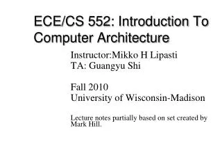
ECE/CS 552: Pipelining to Superscalar. Instructor: Mikko H Lipasti Fall 2010 University of Wisconsin-Madison Lecture notes based on notes by John P. Shen Updated by Mikko Lipasti. Pipelining to Superscalar. Forecast Real pipelines IBM RISC Experience The case for superscalar

E N D
ECE/CS 552: Pipelining to Superscalar Instructor: Mikko H Lipasti Fall 2010 University of Wisconsin-Madison Lecture notes based on notes by John P. Shen Updated by Mikko Lipasti
Pipelining to Superscalar • Forecast • Real pipelines • IBM RISC Experience • The case for superscalar • Instruction-level parallel machines • Superscalar pipeline organization • Superscalar pipeline design
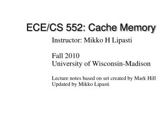
MIPS R2000/R3000 Pipeline Separate Adder
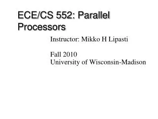
Intel i486 5-stage Pipeline Prefetch Queue Holds 2 x 16B ??? instructions
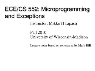
IBM RISC Experience [Agerwala and Cocke 1987] • Internal IBM study: Limits of a scalar pipeline? • Memory Bandwidth • Fetch 1 instr/cycle from I-cache • 40% of instructions are load/store (D-cache) • Code characteristics (dynamic) • Loads – 25% • Stores 15% • ALU/RR – 40% • Branches & jumps – 20% • 1/3 unconditional (always taken) • 1/3 conditional taken, 1/3 conditional not taken
IBM Experience • Cache Performance • Assume 100% hit ratio (upper bound) • Cache latency: I = D = 1 cycle default • Load and branch scheduling • Loads • 25% cannot be scheduled (delay slot empty) • 65% can be moved back 1 or 2 instructions • 10% can be moved back 1 instruction • Branches & jumps • Unconditional – 100% schedulable (fill one delay slot) • Conditional – 50% schedulable (fill one delay slot)
CPI Optimizations • Goal and impediments • CPI = 1, prevented by pipeline stalls • No cache bypass of RF, no load/branch scheduling • Load penalty: 2 cycles: 0.25 x 2 = 0.5 CPI • Branch penalty: 2 cycles: 0.2 x 2/3 x 2 = 0.27 CPI • Total CPI: 1 + 0.5 + 0.27 = 1.77 CPI • Bypass, no load/branch scheduling • Load penalty: 1 cycle: 0.25 x 1 = 0.25 CPI • Total CPI: 1 + 0.25 + 0.27 = 1.52 CPI
More CPI Optimizations • Bypass, scheduling of loads/branches • Load penalty: • 65% + 10% = 75% moved back, no penalty • 25% => 1 cycle penalty • 0.25 x 0.25 x 1 = 0.0625 CPI • Branch Penalty • 1/3 unconditional 100% schedulable => 1 cycle • 1/3 cond. not-taken, => no penalty (predict not-taken) • 1/3 cond. Taken, 50% schedulable => 1 cycle • 1/3 cond. Taken, 50% unschedulable => 2 cycles • 0.20 x [1/3 x 1 + 1/3 x 0.5 x 1 + 1/3 x 0.5 x 2] = 0.167 • Total CPI: 1 + 0.063 + 0.167 = 1.23 CPI
Simplify Branches • Assume 90% can be PC-relative • No register indirect, no register access • Separate adder (like MIPS R3000) • Branch penalty reduced • Total CPI: 1 + 0.063 + 0.085 = 1.15 CPI = 0.87 IPC 15% Overhead from program dependences
Instructions Cycles Time = X X Instruction Program Cycle (code size) (CPI) (cycle time) Processor Performance Time Processor Performance = --------------- • In the 1980’s (decade of pipelining): • CPI: 5.0 => 1.15 • In the 1990’s (decade of superscalar): • CPI: 1.15 => 0.5 (best case) Program
Revisit Amdahl’s Law • h = fraction of time in serial code • f = fraction that is vectorizable • v = speedup for f • Overall speedup: N No. of Processors h 1 - h f 1 - f 1 Time
Revisit Amdahl’s Law • Sequential bottleneck • Even if v is infinite • Performance limited by nonvectorizable portion (1-f) N No. of Processors h 1 - h f 1 - f 1 Time
Pipelined Performance Model • g = fraction of time pipeline is filled • 1-g = fraction of time pipeline is not filled (stalled)
Pipelined Performance Model N Pipeline Depth 1 g 1-g • g = fraction of time pipeline is filled • 1-g = fraction of time pipeline is not filled (stalled)
Pipelined Performance Model • Tyranny of Amdahl’s Law [Bob Colwell] • When g is even slightly below 100%, a big performance hit will result • Stalled cycles are the key adversary and must be minimized as much as possible N Pipeline Depth 1 g 1-g
Motivation for Superscalar[Agerwala and Cocke] Speedup jumps from 3 to 4.3 for N=6, f=0.8, but s =2 instead of s=1 (scalar) Typical Range
Superscalar Proposal • Moderate tyranny of Amdahl’s Law • Ease sequential bottleneck • More generally applicable • Robust (less sensitive to f) • Revised Amdahl’s Law:
Superscalar Proposal • Go beyond single instruction pipeline, achieve IPC > 1 • Dispatch multiple instructions per cycle • Provide more generally applicable form of concurrency (not just vectors) • Geared for sequential code that is hard to parallelize otherwise • Exploit fine-grained or instruction-level parallelism (ILP)
Classifying ILP Machines [Jouppi, DECWRL 1991] • Baseline scalar RISC • Issue parallelism = IP = 1 • Operation latency = OP = 1 • Peak IPC = 1
Classifying ILP Machines [Jouppi, DECWRL 1991] • Superpipelined: cycle time = 1/m of baseline • Issue parallelism = IP = 1 inst / minor cycle • Operation latency = OP = m minor cycles • Peak IPC = m instr / major cycle (m x speedup?)
Classifying ILP Machines [Jouppi, DECWRL 1991] • Superscalar: • Issue parallelism = IP = n inst / cycle • Operation latency = OP = 1 cycle • Peak IPC = n instr / cycle (n x speedup?)
Classifying ILP Machines [Jouppi, DECWRL 1991] • VLIW: Very Long Instruction Word • Issue parallelism = IP = n inst / cycle • Operation latency = OP = 1 cycle • Peak IPC = n instr / cycle = 1 VLIW / cycle
Classifying ILP Machines [Jouppi, DECWRL 1991] • Superpipelined-Superscalar • Issue parallelism = IP = n inst / minor cycle • Operation latency = OP = m minor cycles • Peak IPC = n x m instr / major cycle
Superscalar vs. Superpipelined • Roughly equivalent performance • If n = m then both have about the same IPC • Parallelism exposed in space vs. time