The Production Process and Costs
360 likes | 845 Views
The Production Process and Costs. Production Analysis. Production Function Q = f(K,L) Describes available technology and feasible means of converting inputs into maximum level of output, assuming efficient utilization of inputs:

The Production Process and Costs
E N D
Presentation Transcript
Production Analysis • Production Function Q = f(K,L) • Describes available technology and feasible means of converting inputs into maximum level of output, assuming efficient utilization of inputs: • ensure firm operates on production function (incentives for workers to put max effort) • use cost minimizing input mix • Short-Run vs. Long-Run (increases with capital intensity) • Fixed vs. Variable Inputs
Total Product • Cobb-Douglas Production Function • Example: Q = f(K,L) = K.5 L.5 • K is fixed at 16 units. • Short run production function: Q = (16).5 L.5 = 4 L.5 • Production when 100 units of labor are used? Q = 4 (100).5 = 4(10) = 40 units
Marginal Product of Labor • Continuous case: MPL = dQ/dL • Discrete case: arc MPL = DQ/DL • Measures the output produced by the last worker. • Slope of the production function
Average Product of Labor • APL = Q/L • Measures the output of an “average” worker. • Slope of the line from origin onto the production function
Three significant points are: Max MPL(TP inflects) Max APL = MPL MPL = 0(Max TP) A line from the origin is tangent to Total Product curve at the maximum average product. Law of Diminishing Returns (MPs) TP increases at an increasing rate (MP > 0 and ) until inflection , continues to increase at a diminishing rate (MP > 0 but ) until max and then decreases (MP < 0). Increasing MP Diminishing MP Negative MP
Optimal Level of Inputs Demand for labor Marginal Principle: continue to hire as long as marginal benefit > marginal cost of the input, stop when MB = MC. MC (Pinput, monetary units): cost of hiring the last unit of input. MB (MPinput, physical units): contribution of the last unit of input hired to the total product. MB (VMPinput, monetary units): value of the output produced by the last unit of input = MPinput * Poutput . Downward sloping portion of the VMP curve is the demand for input. Q PL L L* VMPL Solve the following equation for L*: MBL = VMPL = MPL*PQ = PL = MCL
The Long Run Production Function: Q = 10K1/2L1/2
Isoquant • The combinations of inputs (K, L) that yield the producer the same level of output. • The shape of an isoquant reflects the ease with which a producer can substitute among inputs while maintaining the same level of output. • Slope or Marginal Rate of Technical Substitution can be derived using total differential of Q=f(K,L) set equal to zero (no change in Q along an isoquant)
Cobb-Douglas Production Function • Q = KaLb • Inputs are not perfectly substitutable (slope changes along the isoquant) • Diminishing MRTS: slope becomes flatter • Most production processes have isoquants of this shape • Output requires both inputs K-K1 || -K2 Q3 Increasing Output Q2 Q1 L1 < L2 L
K Increasing Output Q2 Q3 Q1 L Linear Production Function • Q = aK + bL • Capital and labor are perfect substitutes (slope of isoquant is constant)y = ax + bK = Q/a - (b/a)L • Output can be produced using only one input
Q3 K Q2 Q1 Increasing Output Leontief Production Function • Q = min{aK, bL} • Capital and labor are perfect complements and cannot be substituted (no MRTS <=> no slope) • Capital and labor are used in fixed-proportions • Both inputs needed to produce output
Isocost K New Isocost for an increase in thebudget (total cost). • The combinations of inputs that cost the same amount of moneyC = K*PK + L*PL • For given input prices, isocosts farther from the origin are associated with higher costs. • Changes in input prices change the slope (Market Rate of Substitution) of the isocost lineK = C/PK - (PL/PK)L C0 C1 L K New Isocost for a decrease in the wage (labor price). L
-PL/PK < -MPL/MPKMPK/PK< MPL/PL K Point of Cost Minimization-PL/PK = -MPL/MPKMPK/PK= MPL/PL -PL/PK > -MPL/MPKMPK/PK> MPL/PL Q L Long Run Cost Minimization Min cost where isocost is tangent to isoquant (slopes are the same) Expressed differently: MP (benefit) per dollar spent (cost) must be equal for all inputs
Returns to Scale Return (MP): How TP changes when one input increases RTS: How TP changes when all inputs increase by the same multiple λ > 0 Q = f(K, L) Q = 50K½L½Q = 100,000 + 500L + 100KQ = 0.01K3 + 4K2L + L2K + 0.0001L3
Expansion path and Long-Run Total Cost K*PK + L*PL = Long-Run Total Cost is the least cost combination of inputs for each production quantity (derives from the expansion path)
Effect of a Fixed Input on Cost of Production • In the short run K is fixed at K0. • Any input L other than L0 will result in other than least TC. • If I1 is required, input L will be reduced to point E, associated with TCmuch higher than optimal at point A.
LTC as a Lower Envelope of STC • Every point on LTC represents a least-cost combination. • In the short run one ormore inputs are fixed so that only a single point on STC is a least-cost combination of inputs. • STC curves intersect cost axis at the value of the TFC.
STC = TFC + TVC = 1000+80Q-6Q2+.2Q3 SAC = STC / Q = TFC/Q + TVC/Q = AFC + AVC AFC = 1000/Q AVC = 80-6Q+.2Q2 SMC = dSTC/dQ = dTFC/dQ + dTVC/dQ = dTVC/dQ = 80-12Q+.6Q2
Productivity of Variable Input and Short-Run Cost = Q = f(L)
Short-Run Total Cost, Total Variable Cost & Total Fixed Cost = TFC + TVC = PL * L = PK * K
LAC as a Lower Envelope of SAC • In the long run all total costs represent least-costs. • All average costs must be least cost as well. • Various short-run cost curves for various values of the fixed input. • In the short run only one point represents least cost. Economies of Scale Diseconomies of Scale Economies of scale (minimum SAC of in the smaller facility greater than SAC in the larger facility) exist up to the minimum LAC (downward sloping portion of LAC curve).Beyond minimum LAC diseconomies of scale.
Long-Run Average Cost and Returns to Scale Diseconomies of Scale Economies of Scale Increasing Returns to Scale: Economies of Scale:Q1 = f(K = 20, L = 10) = 100 PK = 20, PL = 50 LTC1 = 20*20 + 50*10 = 900 LAC1 = 900 / 100 = 9Q2 = f(K = 40, L = 20) = 300 > 2Q2 LTC2 = 20*40 + 50*20 = 1,800 LAC2 = 1,800 / 300 = 6 < LAC1
Economies of Scopeand Cost Complementarity • Cheaper to produce outputs jointly than separately: C(Q1, Q2) < C(Q1, 0) + C(0, Q2) • MC of producing good 1 declines as more of good 2 is produced: MC1 / Q2 < 0 • Example: Joint processing of deposit accounts and loans in banks Scope: Single financial advisor eliminates duplicate common factors of production (computers, loan production offices) Complementarity: Account and credit information developed for deposits lowers credit check and monitoring cost for loans. Expansion of deposit base lowers cost of providing loans.
Quadratic Multi-Product Cost Function • C(Q1, Q2) = f + aQ1Q2 + (Q1 )2 + (Q2 )2 MCi(Qi, Qj) = aQj + 2Qi • Economies of scope (cheaper joint product) if : f > aQ1Q2 C(Q1, 0) + C(0, Q2 ) = f + (Q1)2 + f + (Q2)2 • Cost complementarity exists if: a < 0MCi/ Qj = a < 0
A Numerical Example: • C(Q1, Q2) = 90 - 2Q1Q2 + (Q1 )2 + (Q2 )2 MC1(Q1, Q2) = -2Q2 + 2Q1 • Economies of Scope? Yes, since 90 > -2Q1Q2 • Cost Complementarity? Yes, since a = -2 < 0 • Implications for Merger?