Download
1 / 32
320 likes | 456 Views
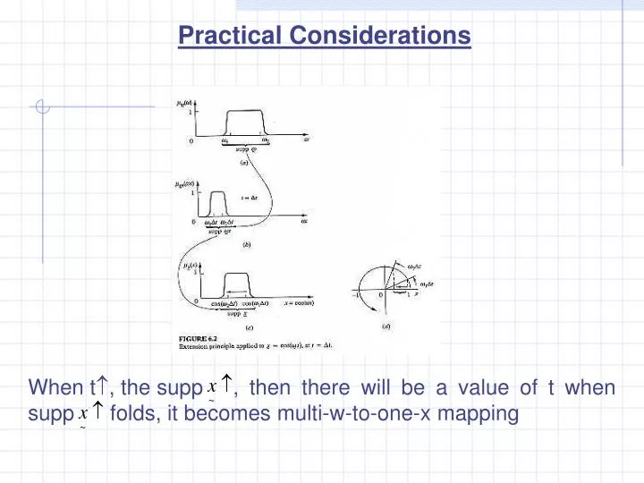
When t , the supp , then there will be a value of t when supp folds, it becomes multi-w-to-one-x mapping. Practical Considerations. Practical Considerations. Then the maximum of all candidate membership value of w is the membership of x.

E N D
When t, the supp , then there will be a value of t when supp folds, it becomes multi-w-to-one-x mapping Practical Considerations
Practical Considerations Then the maximum of all candidate membership value of w is the membership of x.
If supp occupies [-1,1], x [-1,1] in the state of complete fuzziness. Practical Considerations
We define a normal, convex fuzzy set on a real line to be a fuzzy number Let and be fuzzy numbers is a real line in universe Y * Is a set of arithmetic operations Z = * Fuzzy Numbers
Fuzzy Numbers Example:
supp supp (z) = supp * supp = I * J (crisp intervals)! They are intervals! Interval analysis in arithmetic Fuzzy Numbers
I1 = [a,b] a < b I2 = [c,d] c < d I1 * I2 = [a,b] * [c,d] [a b] + [c d] = [a+c b+d] [a b] – [c d] = [a-d b-c] [a b] [c d] = [min(ac,ad,bc,bd) max(ac,ad,bc,bd)] [a b] ÷ [c d] = [a b] [1/d 1/c] 0 [c,d] [a b] > 0 [a b] = [b a] > 0 I(J+K) I J + I K Note: Fuzzy Numbers
Fuzzy Numbers -3[1,2] = [-6,-3] [0,1] – [0,1] = [-1,1] [1,3] [2,4] = [min(1.2,1.4,3.2,3.4) max(1.2,1.4,3.2,3.4)] =[2,1.2] [1 2] ÷ [1 2] = [1 2] [1/2 1] = [1/2 2] If I = [1,2] J = [2,3] K = [1,4] I (J-K) = [1,2] [-2,2] = [-4,4] IJ – IK = [1,2][2,3] – [1,2][1,4] = [2,6] – [1,8] = [-6,5] [-4,4] [-6,5]
Approximate Methods of Extension When discretization of continuous-valued function, it may have irregular and error membership values, which will be propagated from input to output by extension principle. To overcome the above problem, several methods are studied.
Vertex Method Combining the -cut and standard interval analysis. For We can decompose A into a series of -cut and standard interval I. If f(x) is continuous and monotonic on I = [a,b] the interval representing at a particular . B = f(I) = [min(f(a),f(b)) max(f(a),f(b))] Approximate Methods of Extension
Approximate Methods of Extension If y = f(x1,x2,…,xn) Each input variable can be described by an interval Ii Ii = [ai bi] i = 1,2,…,n
Approximate Methods of Extension As seen in the fig. above, the endpoint pairs of each interval intersect in the 3D space and form the vertices (corners) of the Cartesian space. The coordinates of these vertices are the values used in the vertex method when determining the output interval for each -cut. The number of vertices, N, is a quantity equal to N = 2n, where n is the number of fuzzy input variables. When the mapping y = f(x1,x2,…,xn) is continuous in the n-dimensional Cartesian region
Approximate Methods of Extension If there are extreme points where j = 1,2,…,N and k = 1,2,…,m for m extreme points in the region.
Approximate Methods of Extension Example: We wish to determine the fuzziness in the output of a simple nonlinear mapping given by the expression, y = f(x) = x(2 – x), seen in the fig 6.7a, where the fuzzy input variable, x, has the membership function shown in fig 6.7b.
Approximate Methods of Extension We shall solve this problem using the fuzzy vertex method at three -cut levels, for = 0+,0.5,1. As seen in fig 6.7b, the intervals corresponding to these -cuts are I0 = [0.5,2], I0.5 = [0.75,1.5], I1 = [1,1] (a single point).
DSW Algorithm • Select a , 0 < < 1 • Find the interval(s) in the input membership function(s) corresponding to . • Using standard binary interval operations, compute the interval for the output membership function for the selected -cut. • Repeat 1 – 3 for different values of • Example:
DSW Algorithm Example 2: Suppose the domain of the input variable x is changed to include negative numbers… the computations for each -cut will be as follows: Note: The zero marked with the arrow is taken as the minimum, since (-0.5)2 > 0; because zero is contained in the interval [-0.5,1] the minimum of squares of any number in the interval will be zero.
Restricted DSW Algorithm I = [a,b] J = [c,d] a,b,c,d > 0 No Subtraction Then, I J = [a,b] [c,d] = [a c,b d] I/J = [a,b] ÷ [c,d] = [a/d,b/c]
Fuzzy Vectors Formally, a vector, , is called a fuzzy vector if for any element we have 0 < aI< 1 for I = 1,2,…,n. Similarly, the transpose of a fuzzy vector ,denoted by, is a column vector if is a row vector, i.e.,
Fuzzy Vectors Let us define and as fuzzy vectors of length n, and define as the fuzzy inner product of the two fuzzy vectors and as the fuzzy outer product of the two vectors
Fuzzy Vectors Example: Find the inner and outer product of the given fuzzy vectors of length 4 Note: outer product is different from the one in inner algebra.