Induction Variables
This document provides a comprehensive overview of region-based analysis in flow graphs, focusing on the construction and reduction of regions through T1-T2 transformations. It details the criteria for defining a region, self-loop removal, and node combining, as well as the method for computing transfer functions associated with those regions. The analysis employs inductive reasoning to demonstrate that every constructed set of nodes and edges forms a valid region, while also addressing the meet of transfer functions and their closure. Practical examples illustrate these concepts, enhancing understanding.


Induction Variables
E N D
Presentation Transcript
Induction Variables Region-Based AnalysisMeet and Closure of Transfer FunctionsAffine Functions of Reference Variables Jeffrey D. Ullman Stanford University
Regions • A set of nodes N and edges E is a regionif: • There is a header h in N that dominates all nodes in N. • If n≠h is in N, then all predecessors of n are also in N. • I.e., the header is the sole entry into the region. • E consists of all edges between nodes in N, possibly excluding nodes that enter h from somewhere in N. • Note: Every node is a region by itself.
T1-T2 Reduction • For reducible flow graphs, we can “reduce” the graph by two region-creating transformations. • T1: Remove a self-loop from a node. • T2: combine two nodes n and m such that m’s only predecessor is n, and m is not the entry. • Say “n consumes m.” n m
T2 T2 Example: T1-T2 Reduction 1 2 4 3 5
T1 Example: T1-T2 Reduction 14 23 5
T2 Example: T1-T2 Reduction 14 23 5
T2 Example: T1-T2 Reduction 1234 5
T1 Example: T1-T2 Reduction 12345
Example: T1-T2 Reduction 12345
Regions Constructed During T1-T2 Reduction • As we reduce, each node represents a region of the original flow graph, and each edge represents one or more edges of the original flow graph. • T2: Take the union of the two regions represented by the two nodes, plus all edges represented by the edge between them. • T1: Add (to the region represented by the node) those edges represented by the loop that was removed.
Regions Constructed – (2) • Easy inductive proof: every set of nodes and edges constructed is a region. • Key point: When you use T2, the header of the resulting region is the header of the region that consumes the other.
Example: T1-T2 Reduction 1 2 4 3 5
Region-Based Analysis • First, compute for each region, smallest-to-largest, some transfer functions: • For region R constructed by T2 from S consuming T: fR,IN[S] = identity function; fR,IN[T]= meet over paths from the beginning of the header of R to the beginning of the header of T, going only through S. • For region R with header h constructed from S by T1: fR,IN[S] = meet over paths within R from h to h. • For each region R with exit block ( = has an out-edge not in R) B, fR,OUT[B] = meet over paths within R from header of R to end of B.
fU,IN[S]= f1 fS,OUT[2] = f2(f3f2)* f U,OUT[4] = f1f4 fU,OUT[2] = f1f2(f3f2)* Example: Transfer Functions Like regular expressions. = f2 ∧ f2f3f2 ∧f2f3f2f3f2 ∧ .. . . U S 1 2 4 3 5
Additional Assumptions • We can compute the meet of transfer functions: [f ∧g](x) = f(x) ∧ g(x). • Needed when we combine transfer functions from header to several exits. • We can compute the closure f* for each transfer function f, given by f* = f0∧ f1∧ f2∧ … • Note f0 = identity, f1 = f, f2= f composed with f, etc.. • Needed when we apply T1 to consume a back edge.
f(x) Example: RD’s • Meet of transfer functions f(x) = (x - K) ∪ G and g(x) = (x - K’) ∪ G’ corresponds to the paths of f and g in parallel. • Thus, [f∧g](x) = (x – (K ∩K’)) ∪ (G ∪ G’). • f*(x) = x ∪ f(x) ∪ f(f(x)) ∪ … = x ∪ (x – K) ∪ G ∪ ((x - K ∪ G) – K) ∪ G … = x ∪ G. f(f(x))
fV,IN[5] = f1f4 ∧f1f2(f3f2)* fU,OUT[4] = f1f4 fU,OUT[2] = f1f2(f3f2)* Example: Meet Region U consumes node 5 to make region V. V U 1 2 4 3 5
Region-Based Analysis: Basis • If R is a region consisting of a single node (block), and f is the transfer function for that block, thenfR,OUT[R] = f. • Note: we use the same name for the block and the region consisting of only that block.
Region-Based Analysis: Induction • Apply T2: region R consumes region S to make T. • fT,IN(R)= the identity function. • fT,IN(S) = meet of fR,OUT[B] for all predecessors B of the header of S. • For blocks B in R, fT,OUT[B] = fR,OUT[B]. • For blocks B in S, fT,OUT[B] = fT,IN(S) fS,OUT[B].
Induction – (2) • Apply T1: add back edges to region S to make R. • Compute g = meet of fS,OUT[B] for all predecessors B of the header of S. • fR,IN[S] = g*. • Notice that the headers of R and S are the same node, but there are paths within R that are not in S, yet take you to the header of S. • For all blocks B in S (and therefore in R) let fR,OUT[B] = fR,IN[S]fS,OUT[B].
Now We Work Large-to-Small • Let e be the header of the region that is the entire flow graph. • Start with IN(e) = vENTRY. • Proceed inward, from larger regions to smaller. • If R was constructed from S by T1, and both have header h, replace IN(h) by fR,IN(S)(IN(h)). • If T, with header h’ was constructed from R and S, with R consuming S, and S has header h, initialize IN(h) to fT,IN(S)(IN(h’).
IN[1] = fR,IN[V](vENTRY) = f*V,OUT[5] ](vENTRY) Examples: Top-Down Finale 1 2 4 U V R 3 5 IN[5] = fV,IN[5](IN(1))
New Topic: Symbolic Analysis • Values V are mappings from variables to expressions involving reference variables. • Example: m(a) = 2i; m(b) = i + j + 1. • i and j are the reference variables. • We are going to deal with two complicated types of functions: • Mappings from variables to expressions, as above. • Transfer functions from mappings (in) to mappings (out).
Application to Induction Variables • Reference variables are basic induction variables= counts of the number of times around some loop. • This count is well-defined for “natural loops.” • Set of values V for the framework = affine mappings= each variable is mapped to either: • A linear function of the reference variables, or • NAA = “Not an affine” mapping, or • UNDEF = top element = “nothing known.”
Example: Affine Mapping m(a) = 2i + 3j + 4 m(b) = NAA m(c) = 4i + 1 m(d) = UNDEF
Lattice for Each Variable UNDEF Less Ignorance All affine functions of reference variables NAA Note: The lattice for V is the product of one of these for each variable.
Induction Variable Discovery • Natural application of region-based analysis. • Each loop is a region, and its induction variables can be discovered by a framework based on affine mappings.
Example: A Transfer Function • Let f be the transfer function associated with a block containing only a = a+10. • Let m be the input mapping for the block; then f(m) = m’, where: • m’(a) = m(a) + 10. • m’(x) = m(x) for all x ≠a. • Book uses the notation f(m)(a) = m(a) + 10, etc., to avoid having to name f(m). m Question: What if m(a) is NAA or UNDEF? a = a + 10 m'
The Meet Operator • (f ∧ g)(m)(x) = • f(m)(x) if f(m)(x) = g(m)(x). • f(m)(x) if g(m)(x) = UNDEF. • g(m)(x) if f(m)(x) = UNDEF. • NAA otherwise.
R (a) = m(a) (b) = m(a)+2 fB3(m) (a) = m(a)+5 (b) = m(b) fB2(m) (a) = m(b)+3 (b) = m(b) fB4(m) (a) = m(a)+5 (b) = m(a)+2 fR,OUT[B4](m) Example: Some Analysis B1 B3 b=a+2 a=a+5 B2 B4 a=b+3 B5
R (a) = m(a)+5 (b) = m(b) fB2(m) (a) = m(a)+5 (b) = m(a)+2 fR,OUT[B4](m) (a) = m(a)+5 (b) = NAA fS,OUT[B5](m) Example: Meet S B1 B3 b=a+2 a=a+5 B2 B4 a=b+3 B5
Handling Loop Regions • Treat the iteration count i as a basic induction variable. • If f(m)(x) = m(x)+c, then fi(m)(x) = m(x)+ci. • Some other cases, e.g., where m(x) is an affine function of basic induction variables, in book.
(a) = m(a)+5i (b) = NAA fS,OUT[B5](m) (a) = m(a)+5i (b) = m(a)+5i+2 OUTi[B3](m) (a) = m(a)+5i+5 (b) = NAA OUTi[B2](m) (a) = m(a)+5i+5 (b) = m(a)+5i+2 OUTi[B4](m) (a) = m(a)+5i+5 (b) = NAA OUTi[B5](m) Example: The Entire Loop i T B1 B3 b=a+2 S a=a+5 B2 a=b+3 B4 B5 (a) = m(a)+5 (b) = NAA fS,OUT[B5](m)
Taking Advantage of Affine Expressions • Replace the loop counter variable by one of the induction variables (variables that are mapped to an affine expression of the loop count at the point were the loop count is tested).
Here, the value of a is m(a)+5i, where m(a) is the value of a before entering the loop, and i is the number of iterations of the loop so far. If i is dead on exit from the loop, delete “i=i+1” and “i=0”. Example: Assume i is Loop Counter i=0 a=30 B1 i<10? Since a=30 when i=0, replace “i<10?” by “a<80?”. B3 b=a+2 a=a+5 B2 B4 a=b+3 And since i is an induction variable, if not dead we can just assign i = 10 at the exit. i=i+1 B5
Example: Revised Code a=30 B1 a<80? B3 b=a+2 a=a+5 B2 B4 a=b+3 B5