Examining the Sensitivity of the CM1 Model to Initial Potential Temperature Perturbations
This study investigates the sensitivity of the CM1 cloud-resolving model, created by George Bryan at NCAR, to variations in initial potential temperature perturbations. Utilizing a 3D, non-hydrostatic, and non-linear approach, the research explores the implications of temperature anomalies on storm cell dynamics, particularly focusing on how changes in the maximum temperature perturbation and warm bubble radius influence storm behavior. Results indicate that increases in potential temperature perturbation lead to earlier cell splitting and enhanced updraft strength, highlighting the model's sensitivity to these parameters.

Examining the Sensitivity of the CM1 Model to Initial Potential Temperature Perturbations
E N D
Presentation Transcript
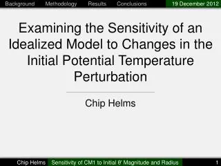
Examining the Sensitivity of an Idealized Model to Changes in the Initial Potential Temperature Perturbation Chip Helms
Background The Idealized Model: CM1 • Created by George Bryan (NCAR) • 3D, non-hydrostatic, non-linear, cloud-resolving, idealized model • No data assimilation • Uses a horizontally constant field for the base state • Adds perturbations to base state • e.g. warm bubble, cold blob, forced convergence • Benefits of using CM1 • Conserves mass and energy better than other modern cloud models • Faster and uses less memory than other models for idealized studies • Very flexible, can be used for a large variety of studies
Goal • Qualitatively examine CM1 sensitivity to: • Initial maximum magnitude of θ' • Initial horizontal warm bubble radius • Potential implications of study: • Sensitivity of cloud-resolving models to temperature anomalies • e.g. magnitude and extent of an urban heat island
Methodology Methodology • Two sets of runs to test sensitivities
Methodology Model Settings
Results Sensitivity to magnitude of θ' Composite Reflectivity Cell split occurs earlier as θ' increases
Results Sensitivity to Warm Bubble Radius Cell split occurs earlier as radius increases Cell splitting is related to the interaction between vorticity and updrafts Look at updraft strength evolution
Results Delay in reaching peak updraft strength is non-linear function of θ' 2.0 K 1.0 K 1.5 K 0.5 K
Results Relatively low sensitivity at 7 km radius and above Model Dispersion 2-6Δx 2-6 km radii Relatively high sensitivity at 6 km radius and below
Conclusions Conclusions • As θ' or warm bubble radius increases, storm cell splits earlierand reaches peak updraft strength earlier • More sensitive to θ' than radius • Small warm bubble radius runs have resolution and dispersion issues • Impacts 5 km radius most • Very little sensitivity at or above 7 km • Suggests sensitivity is due to model dispersion
Conclusions Peak Updraft Limit • Function of CAPE CAPE = 1946 wmax= 62 m/s • Actual < 55 m/s • Difference due to assumptions of CAPE
Methodology Initial Background Conditions Hodograph corresponds to these levels
Methodology Hodograph Refresher • Trace of wind vector direction (azimuth) and magnitude (radius) • Straight hodographs suggest cells will split • Veering (backing) hodographs suggest right (left) cell will be dominant
Methodology Model Settings - Continued • Boundary conditions: • Open-radiativelateral boundary conditions • Zero-flux top/bottom boundary conditions • Not included in these runs: • Atmospheric radiation • Surface drag • Surface fluxes
Conclusions Outlying Model Runs • θ' = 0.5K lags behind other runs • Radius = 5 km lags significantly behind other runs • Possibly due to turbulent mixing having a greater impact on tight gradients • smaller size of anomaly would be diffused faster • Could also be due to dampening near the 2Δx scale (recall Δx = 2 km)
Detailed model settings • 5th order horizontal/vertical advection schemes • Negative moisture is corrected by taking moisture from adjacent grid cells • No additional artificial diffusion beyond subgrid turbulence scheme • Sixth order diffusion scheme (coefficient = 0.040) • TKE subgrid turbulence scheme • Zero flux boundary condition for vertical diffusion of winds/scalars at top/bottom of domain • Uses Rayleigh damping at upper levels (e-fold time = 1/300, applied above 14km), but not near horizontal boundaries • Uses Klemp-Wilhelmson time-splitting, vertically implicit pressure solver (as in MM5, ARPS, WRF), coeff for divergence damper = 0.10, slight foreward-in-time bias used for vertically implicit acoustic solver (alpha = 0.60) • Moisture scheme: Morrison double-moment scheme • Hail is used for large ice category • cloud droplet concentration: 250 cm^-3 (marine=100,continental=300) • No Coriolis force • Includes dissipative heating • No energy fallout term • Open-radiative lateral boundary scheme: Durran-Klemp (1983) formulation • Initial base-state sounding: Weisman-Klemp analytic sounding • Initial base-state wind profile: RKW-type profile • Initial pressure perturbation is zero everywhere
Results Sensitivity to magnitude of θ' Composite Reflectivity Cell split occurs earlier as θ' increases Cell splitting is related to the interaction between vorticity and updrafts