Download
1 / 44
500 likes | 968 Views
DIMENSIONAL ANALYSIS. SECTION 5. Dimensions and units. Any physical situation can be described by certain familiar properties e.g. length, velocity, area, volume, acceleration etc. These are all known as dimensions.

E N D
DIMENSIONAL ANALYSIS SECTION 5
Dimensions and units Any physical situation can be described by certain familiar properties e.g. length, velocity, area, volume, acceleration etc. These are all known as dimensions. Of course dimensions are of no use without a magnitude being attached. We must know more than that something has a length. It must also have a standardised unit - such as a meter, a foot, a yard etc. Dimensions are properties which can be measured. Units are the standard elements we use to quantify these dimensions. In dimensional analysis we are only concerned with the nature of the dimension i.e. its quality not its quantity. The following common abbreviation are used:
Dimensions and units • length = L • mass = M • time = T • force = F • temperature = In this module we are only concerned with L, M, T and F (not Q). We can represent all the physical properties we are interested in with L, T and one of M or F (F can be represented by a combination of LTM). These notes will always use the LTM combination.
Dimensions and units The following table (taken from earlier in the course) lists dimensions of some common physical quantities:
Dimensional Homogeneity Any equation describing a physical situation will only be true if both sides have the same dimensions. That is it must be dimensionally homogenous. For example the equation which gives for over a rectangular weir (derived earlier in this module) is,
Dimensional Homogeneity The SI units of the left hand side are m3s The units of the right hand side must be the same. Writing the equation with only the SI units gives
Results of dimensional analysis The result of performing dimensional analysis on a physical problem is a single equation. This equation relates all of the physical factors involved to one another. This is probably best seen in an example. If we want to find the force on a propeller blade we must first decide what might influence this force. It would be reasonable to assume that the force, F, depends on the following physical properties:
Buckingham’s theorems Although there are other methods of performing dimensional analysis, (notably the indicial method) the method based on the Buckingham theorems gives a good generalised strategy for obtaining a solution. This will be outlined below.
Choice of repeating variables Repeating variables are those which we think will appear in all or most of the p groups, and are a influence in the problem. Before commencing analysis of a problem one must choose the repeating variables. There is considerable freedom allowed in the choice.
An example Taking the example discussed above of force F induced on a propeller blade, we have the equation
Common groups During dimensional analysis several groups will appear again and again for different problems. These often have names. You will recognise the Reynolds number rud/m. Some common non-dimensional numbers (groups) are listed below. Reynolds number inertial, viscous force ratio
Similarity • Geometric similarity Geometric similarity exists between model and prototype if the ratio of all corresponding dimensions in the model and prototype are equal.
Similarity • Kinematic similarity
Similarity • Dynamic similarity
Models When a hydraulic structure is build it undergoes some analysis in the design stage. Often the structures are too complex for simple mathematical analysis and a hydraulic model is build. Usually the model is less than full size but it may be greater. The real structure is known as the prototype. The model is usually built to an exact geometric scale of the prototype but in some cases - notably river model - this is not possible. Measurements can be taken from the model and a suitable scaling law applied to predict the values in the prototype.
Models To illustrate how these scaling laws can be obtained we will use the relationship for resistance of a body moving through a fluid. The resistance, R, is dependent on the following physical properties:
Models • Dynamically similar model examples Example 1 An underwater missile, diameter 2m and length 10m is tested in a water tunnel to determine the forces acting on the real prototype. A 1/20th scale model is to be used. If the maximum allowable speed of the prototype missile is 10 m/s, what should be the speed of the water in the tunnel to achieve dynamic similarity? For dynamic similarity the Reynolds number of the model and prototype must be equal:
Models Note that this is a very high velocity. This is one reason why model tests are not always done at exactly equal Reynolds numbers. Some relaxation of the equivalence requirement is often acceptable when the Reynolds number is high. Using a wind tunnel may have been possible in this example. If this were the case then the appropriate values of the r and m ratios need to be used in the above equation.
Models Example 2 A model aeroplane is built at 1/10 scale and is to be tested in a wind tunnel operating at a pressure of 20 times atmospheric. The aeroplane will fly at 500km/h. At what speed should the wind tunnel operate to give dynamic similarity between the model and prototype? If the drag measure on the model is 337.5 N what will be the drag on the plane? From earlier we derived the equation for resistance on a body moving through air:
Models • Models with free surfaces - rivers, estuaries etc. When modelling rivers and other fluid with free surfaces the effect of gravity becomes important and the major governing non-dimensional number becomes the Froude (Fn) number. The resistance to motion formula above would then be derived with g as an extra dependent variables to give an extra p group. So the defining equation is:
Models • Geometric distortion in river models When river and estuary models are to be built, considerable problems must be addressed. It is very difficult to choose a suitable scale for the model and to keep geometric similarity. A model which has a suitable depth of flow will often be far to big - take up too much floor space. Reducing the size and retaining geometric similarity can give tiny depth where viscous force come into play. These result in the following problems: i. accurate depths and depth changes become very difficult to measure; ii. the bed roughness of the channel becomes impracticably small; iii. laminar flow may result - (turbulent flow is normal in river hydraulics.)
Models The solution often adopted to overcome these problems is to abandon strict geometric similarity by having different scales in the horizontal and the vertical. Typical scales are 1/100 in the vertical and between 1/200 and 1/500 in the horizontal. Good overall flow patterns and discharge characteristics can be produced by this technique, however local detail of flow is not well modelled. In these model the Froude number (u2/d) is used as the dominant non-dimensional number. Equivalence in Froude numbers can be achieved between model and prototype even for distorted models. To address the roughness problem artificially high surface roughness of wire mesh or small blocks is usually used.