Understanding Random Variables in Probability: Midterm Scores and Dice Rolls
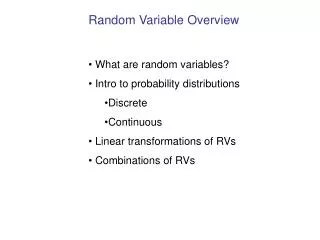
This lecture explores the concept of random variables, defining them as functions that map outcomes from a sample space to real numbers. Through examples such as midterm scores and dice rolls, we illustrate how probabilities are calculated for specific outcomes. The lecture emphasizes the difference between deterministic functions and randomness, illustrating the role of probability mass functions (pmf) and distribution functions in analyzing random variables. By examining these concepts, students gain a fundamental understanding of how to work with random variables in statistical contexts.

Understanding Random Variables in Probability: Midterm Scores and Dice Rolls
E N D
Presentation Transcript
ENGG2012BLecture 18Random variable Kenneth Shum ENGG2012B
Histogram of midterm score ENGG2012B
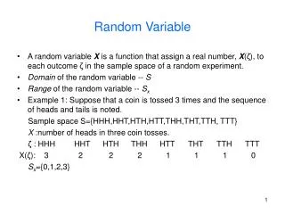
The idea of random variables • Given a sample space and a probability measure defined on it, very often we cannot observe the elements in the sample space directly, but through a function defined on the sample space. • For each , we observe a real number X(). This is a function of . • We would like to calculate the probability of the events such as X() 0, X() = 30, etc. ENGG2012B
Formal definition of RV • A random variable is not a variable. It is a function from the sample space to the real numbers. • There is nothing random in the function itself. The randomness comes from the probability measure assigned to the events of the sample space. • A random variable is often written as X(), where is an element in the sample space. The real line X() ENGG2012B
Example: Midterm score The “midterm score” is a random variable. It maps a student to the corresponding midterm score. Student C 35 Student A 23 Student B Class of ENGG2012B Real line If we randomly pick a student out ofthe total of 90 students, the probabilitythat “midterm score = 23” is 2/90. ENGG2012B
Example: dart Note: the associationof a point on the dartboardand the score is completelydeterministic. The randomnessonly comes from throwingthe random dart. • In the random experiment of rowing a dart randomly to a circle of radius 3, let X() be the score defined by • X() = 3 if the distance to the center is less than 1. • X() = 2 if the distance to the center is between 1 and 2. • X() = 1 if the distance to the center is between 2 and 3. dartboard 3 2 Pr( X() = 3) = 12 / (32) = 1/9 Pr(X() = 2) = ( 22 –12)/ (32) =1/3 1 Pr(X() = 1) = ( 32 –22)/ (32)=5/9 ENGG2012B
Notations • The probability function Pr is sometime regarded as a operator, which takes an event as input and outputs a real number. • If we want to emphasize that “Pr” is a function with events as input, we shall write for the probability of X() = 1, or simply ENGG2012B
Probability distribution function • Sometimes, we underlying sample space is very complicated or very large. We only care about the distribution of the random variable, but not sample space . • We may try to forget the sample space and work with the probability mass function (pmf), f(i) = Pr(X() = i). • If we want to emphasize that it is the pmf of random variable X(), we can write fX(i). • The pmf is sometimes called the “distribution of X”. However, in probability, the term “distribution” usually refers to something else, namely, F(z) = Pr(X() z). • In the remainder of this lecture, we assume that the random variables take values in the integers, i.e., i is an integer. ENGG2012B
Example: sum of two dice • Roll two fair dice. Let X() be the sum. The pmf of X() can be tabulated as follows. The sample spaceconsists of 36 outcomes ENGG2012B
Example: number of heads • Toss 5 fair coins. Let Y() be the number of heads. The pmf of Y() in tabular form is ENGG2012B