Understanding NP & NP-Complete Problems in Algorithm Analysis
260 likes | 370 Views
Learn about P, NP, and NP-Complete classes of problems, complexity classes, graph theory concepts, and the relation among P, NP, and NPC. Also, explore decision vs. optimization problems and their significance in algorithm analysis.

Understanding NP & NP-Complete Problems in Algorithm Analysis
E N D
Presentation Transcript
Analysis of Algorithms NP & NP-Complete Prof. Muhammad Saeed
Classes Of Problems 1. P 2. NP 3. NP-Complete (NPC, NP-C) Analysis OF Algorithms NP-NP-Complete Page
…… Classes Of Problems • P: • Consists of those problems that are solvable in polynomial time. More specifically, they are problems that can be solved in time O(nk) for some constant k, where n is the size of the input to the problem. They are called easy or tractable. Problems that require superpolynomial time as being intractable, or hard. • NP: • Consists of those problems that are verifiable in polynomial time, it means if we were somehow given a ‘certificate’ of a solution, then we could verify that the certificate is correct in polynomial time in the size of the input to the problem. Analysis OF Algorithms NP-NP-Complete Page
NPC (NP-Complete): • Problems in NP and as hard as any problem in NP. No polynomial-time algorithm has yet been discovered for an NP-complete problem, nor has anyone yet been able to prove that no polynomial-time algorithm can exist for any one of them. Analysis OF Algorithms NP-NP-Complete Page
Complexity Class P • Deterministic in nature • Solved by conventional computers in polynomial time • O(1) Constant • O(log n) Sub-linear • O(n) Linear • O(n log n) Nearly Linear • O(n2) Quadratic • O(nk) k-Polynomial • Polynomial upper and lower bounds Analysis OF Algorithms NP-NP-Complete Page
Shortest vs. longest simple paths: Even with negative edge weights, we can find shortest paths from a single source in a directed graph G = (V, E) in O(V E) time. Finding a longest simple path between two vertices is difficult, however. Merely determining whether a graph contains a simple path with at least a given number of edges is NP-complete. Analysis OF Algorithms NP-NP-Complete Page
Euler tour vs. hamiltonian cycle: An Euler tour of a connected, directed graph G = (V, E) is a cycle that traverses each edge of G exactly once, although it may visit a vertex more than once. We can determine whether a graph has an Euler tour in only O(E) time and, in fact, we can find the edges of the Euler tour in O(E) time. A hamiltonian cycle of a directed graph G = (V, E) is a simple cycle that contains each vertex in V. Determining whether a directed graph has a hamiltonian cycle is NP-complete. determining whether an undirected graph has a hamiltonian cycle is NP-complete. Analysis OF Algorithms NP-NP-Complete Page
2-CNF satisfiability vs. 3-CNF satisfiability: A boolean formula contains variables whose values are 0 or 1; boolean connectives such as ∧ (AND), ∨ (OR), and ¬ (NOT); and parentheses. A boolean formula is satisfiable if there is some assignment of the values 0 and 1 to its variables that causes it to evaluate to 1. A boolean formula is in k-conjunctive normal form, or k-CNF, if it is the AND of clauses of ORs of exactly k variables or their negations. For example, the boolean formula (x1 ∨ ¬x2) ∧ (¬x1 ∨ x3) ∧ (¬x2 ∨ ¬x3) is in 2-CNF. (It has the satisfying assignment x1 = 1, x2 = 0, x3 = 1.) There is a polynomial-time algorithm to determine whether a 2-CNF formula is satisfiable, a 3-CNF formula is satisfiable is NP-complete. Analysis OF Algorithms NP-NP-Complete Page
Relation among P, NP, NPC • P NP (Sure) • NPC NP (sure) • P = NP (or P NP, or P NP) ??? • NPC = NP (or NPC NP, or NPC NP) ??? • P NP: one of the deepest, most perplexing open research problems in (theoretical) computer science since 1971. • Any problem in P is also in NP, since if a problem is in P then we can solve it in polynomial time without even being given a certificate. • Most theoretical computer scientists believe that NPC is intractable (i.e., hard, and P NP). Analysis OF Algorithms NP-NP-Complete Page
View of Theoretical Computer Scientists on P, NP, NPC NPC NP P P NP, NPC NP, P NPC = Analysis OF Algorithms NP-NP-Complete Page
Why discussion on NPC • If a problem is proved to be NPC, a good evidence for its intractability (hardness). • Not waste time on trying to find efficient algorithm for it • Instead, focus on design approximate algorithm or a solution for a special case of the problem • Some problems looks very easy on the surface, but in fact, is hard (NPC). Analysis OF Algorithms NP-NP-Complete Page
Decision VS. Optimization Problems • Decision problem: solving the problem by giving an answer “YES” or “NO” • Optimization problem: solving the problem by finding the optimal solution. • Examples: • SHORTEST-PATH (optimization) • Given G, u,v, find a path from u to v with fewest edges. • PATH (decision) • Given G, u,v, and k, whether exist a path from u to v consisting of at most k edges. Analysis OF Algorithms NP-NP-Complete Page
Decision VS. Optimization Problems (Cont.) • Decision is easier (i.e., no harder) than optimization • If there is an algorithm for an optimization problem, the algorithm can be used to solve the corresponding decision problem. • Example: SHORTEST-PATH for PATH • If optimization is easy, its corresponding decision is also easy. Or in another way, if provide evidence that decision problem is hard, then the corresponding optimization problem is also hard. • NPC is confined to decision problem. (also applicable to optimization problem.) • Another reason is that: easy to define reduction between decision problems. Analysis OF Algorithms NP-NP-Complete Page
(Poly) reduction between decision problems • Problem (class) and problem instance • Instance of decision problem A and instance of decision problem B • A reduction from A to B is a transformation with the following properties: • The transformation takes poly time • The answer is the same (the answer for is YES if and only if the answer for is YES). Analysis OF Algorithms NP-NP-Complete Page
Implication of (poly) reduction YES YES (Poly) Reduction Algorithm for B NO Decision algorithm for A NO • If decision algorithm for B is poly, so does A. • A is no harder than B (or B is no easier than A) 2. If A is hard (e.g., NPC), so does B. 3. How to prove a problem B to be NPC ?? (at first, prove B is in NP, which is generally easy.) 3.1 find a already proved NPC problem A Question: What is and how to prove the first NPC problem? Circuit-satisfiability problem. Analysis OF Algorithms NP-NP-Complete Page
Travelling Salesman Problem (TSP) • For each two cities, an integer cost is given to travel from one of the two cities to the other. The salesperson wants to make a minimum cost circuit visiting each city exactly once. Analysis OF Algorithms NP-NP-Complete Page
Circuit-SAT Logic Gates 0 1 0 1 1 NOT 1 1 0 OR 1 0 1 0 1 AND • Take a Boolean circuit with a single output node and ask whether there is an assignment of values to the circuit’s inputs so that the output is “1” Analysis OF Algorithms NP-NP-Complete Page
Two instances of circuit satisfiability problems Analysis OF Algorithms NP-NP-Complete Page
Knapsack 5 6 2 3 4 7 1 L s • Given s and w can we translate a subset of rectangles to have their bottom edges on L so that the total area of the rectangles touching L is at least w? Analysis OF Algorithms NP-NP-Complete Page
5-Clique Analysis OF Algorithms NP-NP-Complete Page
Vertex Cover A graph and its complement. Note that there is a 4-clique (consisting of vertices a, b, d, and f) in the graph on the left. Note also that the vertices not in this clique (namely c and e) do form a cover for the complement of this graph (which appears on the right). Analysis OF Algorithms NP-NP-Complete Page
The Halting Problem • Given an algorithm A and an input I, will the algorithm reach a stopping place? • In general, we cannot solve this problem in finite time. • loop • exit if (x = 1) • if (even(x)) then • x x div 2 • else • x 3 * x + 1 • endloop Analysis OF Algorithms NP-NP-Complete Page
Hamiltonian Path Analysis OF Algorithms NP-NP-Complete Page
Euler tour vs. hamiltonian cycle: An Euler tour of a connected, directed graph G = (V, E) is a cycle that traverses each edge of G exactly once, although it may visit a vertex more than once. We can determine whether a graph has an Euler tour in only O(E) time and, in fact, we can find Analysis OF Algorithms NP-NP-Complete Page
END Analysis OF Algorithms NP-NP-Complete Page