Download
1 / 44
440 likes | 590 Views
SEMINAR 236825 OPEN PROBLEMS IN DISTRIBUTED COMPUTING. Winter 2013-14 Hagit Attiya & Faith Ellen. INTRODUCTION. Distributed Systems. Distributed systems are everywhere: share resources communicate increase performance (speed & fault tolerance) Characterized by

E N D
SEMINAR 236825 OPEN PROBLEMS IN DISTRIBUTED COMPUTING Winter 2013-14 Hagit Attiya & Faith Ellen Introduction
INTRODUCTION Introduction
Distributed Systems • Distributed systems are everywhere: • share resources • communicate • increase performance (speed & fault tolerance) • Characterized by • independent activities (concurrency) • loosely coupled parallelism (heterogeneity) • inherent uncertainty E.g. • operating systems • (distributed) database systems • software fault-tolerance • communication networks • multiprocessor architectures Introduction
Main Admin Issues • Goal: Read some interesting papers, related to some open problems in the area • Mandatory (active) participation • 1 absence w/o explanation • Tentative list of papersalready published • First come first served • Lectures in English Introduction
Course Overview: Basic Models messagepassing sharedmemory PRAM synchronous asynchronous Introduction
Message-Passing Model • processorsp0, p1, …, pn-1 are nodes of the graph. Each is a state machine with a local state. • bidirectional point-to-point channels are the undirected edges of the graph. • Channel from pito pjis modeled in two pieces: • outbufvariable of pi(physical channel) • inbufvariable of pj (incoming message queue) p0 2 1 2 2 p2 p3 p1 1 3 1 1 Introduction
inbuf[1] outbuf[2] p1's local variables p2's local variables outbuf[1] inbuf[2] Modeling Processors and Channels • processorsp0, p1, …, pn-1 are nodes of the graph. Each is a state machine with a local state. • bidirectional point-to-point channels are the undirected edges of the graph. • Channel from pito pjis modeled in two pieces: • outbuf variable of pi(physical channel) • inbufvariable of pj (incoming message queue) Introduction
Configuration A snapshot of entire system: accessible processor states (local variables & incoming msg queues) as well as communication channels. Formally, a vector of processor states (including outbufs, i.e., channels), one per processor Introduction
p1 m3 m2 m1 p2 Deliver Event Moves a message from sender's outbuf to receiver's inbuf; message will be available next time receiver takes a step p1 m3 m2 m1 p2 Introduction
Computation Event Occurs at one processor • Start with old accessible state (local vars + incoming messages) • Apply processor's state machine transition function; handle all incoming messages • End with new accessible state with empty inbufs& new outgoing messages b a old local state new local state c d e Introduction
Execution configuration, event, configuration, event, configuration, … • In the first configuration: each processor is in initial state and all inbufs are empty • For each consecutive triple configuration, event, configurationnew configuration is same as old configuration except: • if delivery event: specified msg is transferred from sender's outbuf to receiver's inbuf • if computation event: specified processor's state (including outbufs) change according to transition function Introduction
Asynchronous Executions • An execution is admissible in asynchronous model if • every message in an outbuf is eventually delivered • every processor takes an infinite number of steps • No constraints on when these events take place: arbitrary message delays and relative processor speeds are not ruled out • Models a reliable system (no message is lost and no processor stops working) Introduction
Example: Simple Flooding Algorithm • Each processor's local state consists of variable color, either red or green • Initially: • p0: color = green, all outbufs contain M • others: color = red, all outbufs empty • Transition: If M is in an inbuf and color = red, then change color to green and send M on all outbufs Introduction
p0 p0 M M M M p2 p1 deliver event at p1from p0 p2 p1 computation event by p1 p0 p0 M M M M computation event by p2 deliver event at p2from p1 p2 p1 p2 p1 M M Example: Flooding Introduction
p0 p0 M M M M M M p2 p1 deliver event at p1from p2 p2 p1 computation event by p1 M M p0 p0 M M M M M M etc. to deliver rest of msgs p2 p1 deliver event at p0from p1 p2 p1 Example: Flooding (cont'd) Introduction
(Worst-Case) Complexity Measures • Message complexity: maximum number of messages sent in any admissible execution • Time complexity: maximum "time" until all processes terminate in any admissible execution. • How to measure time in an asynchronous execution? • Produce a timed executionby assigning non-decreasing real times to events so that time between sending and receiving any message is at most 1. • Time complexity: maximum time until termination in any timedadmissible execution. Introduction
Complexities of Flooding Algorithm A state is terminated if color = green. • One message is sent over each edge in each direction message complexity is 2m, where m = number of edges. • A node turns green once a "chain" of messages reaches it from p0 time complexityis diameter + 1 time units. Introduction
Synchronous Message Passing Systems An execution is admissible for the synchronous model if it is an infinite sequence of rounds • A round is a sequence of deliver events moving all msgs in transit into inbuf's, followed by a sequence of computation events, one for each processor. Captures the lockstep behavior of the model Also implies • every message sent is delivered • every processor takes an infinite number of steps. Timeis the number of rounds until termination Introduction
p0 p0 M M p2 p1 round 1 events p2 p1 round 2 events p0 M M p2 p1 M M Example: Flooding in the Synchronous Model Time complexity is diameter + 1 Message complexity is 2m Introduction
Broadcast Over a Rooted Spanning Tree • Processors have information about a rooted spanning tree of the communication topology • parentand children local variables at each processor • Complexities (synchronous and asynchronous model) • time is depth of the spanning tree, which is at most n - 1 • number of messages is n - 1, since one message is sent over each spanning tree edge • root initially sends M to its children • when a processor receives M from its parent • sends M to its children • terminates (sets a local Boolean to true) Introduction
Finding a Spanning Tree from a Root Introduction • root sends M to all its neighbors • when non-root first gets M • set the sender as its parent • send "parent" msg to sender • send M to all other neighbors (if no other neighbors, then terminate) • when get M otherwise • send "reject" msg to sender • use "parent" and "reject" msgs to set children variables and terminate (after hearing from all neighbors)
c b c b a a f d d f e e g h g h Execution of Spanning Tree Algorithm root root Both models: O(m) messages O(diam) time Asynchronous: not necessarily BFS tree Synchronous: always gives breadth-first search (BFS) tree Introduction
b c b c a a f d d f e e g h g h Execution of Spanning Tree Algorithm root root No! An asynchronous execution gavea depth-first search (DFS) tree.Is DFS property guaranteed? Another asynchronous execution results in this tree: neither BFS nor DFS Introduction
Shared Memory Model Processors (also called processes) communicate via a set of shared variables Each shared variable has a type, defining a set of primitive operations (performed atomically) • read, write • compare&swap(CAS) • LL/SC, DCAS, kCAS, … • read-modify-write (RMW), kRMW p0 p1 p2 read write RMW write X Y Introduction
Changes from the Message-Passing Model Introduction • no inbuf and outbuf state components • configuration includes values for shared variables • one event type: a computation step by a process • pi 's state in old configuration specifies which shared variable is to be accessed and with which primitive • shared variable's value in the new configuration changes according to the primitive's semantics • pi 's state in the new configuration changes according to its old state and the result of the primitive An execution is admissibleif every processor takes an infinite number of steps
data Abstract Data Types • Abstract representation of data & set of methods (operations) for accessing it • Implement using primitives on base objects • Sometimes, a hierarchy of implementations: Primitive operations implemented from more low-level ones Introduction
Executing Operations deq 1 invocation response P1 enq(1) ok P2 enq(2) P3 Introduction
Interleaving Operations, or Not enq(1) ok deq 1 enq(2) Sequential behavior: invocations & responses alternate and match (on process & object) Sequential Specification: All legalsequential behaviors Introduction
Correctness: Sequential consistency [Lamport, 1979] • For every concurrent execution there is a sequential execution that • Contains the same operations • Is legal (obeys the sequential specification) • Preserves the order of operations by the same process Introduction
Example 1: Multi-Writer Registers Using (multi-reader) single-writer registers Add logical time to values Write(v,X) read TS1,..., TSn TSi = max TSj+1 write v,TSi Read only own value Read(X) read v,TSi return v Once in a while read TS1,..., TSn and write to TSi Need to ensure writes are eventually visible Introduction
Timestamps • The timestamps of two write operations by the same process are ordered • If a write operation completes before another one starts, it has a smaller timestamp Write(v,X) read TS1,..., TSn TSi = max TSj+1 write v,TSi Introduction
Multi-Writer Registers: Proof Write(v,X) read TS1,..., TSn TSi = max TSj+1 write v,TSi Read(X) read v,TSi return v Once in a while read TS1,..., TSn and write to TSi • Create sequential execution: • Place writes in timestamp order • Insert reads after the appropriate write Introduction
Multi-Writer Registers: Proof • Create sequential execution: • Place writes in timestamp order • Insert reads after the appropriate write • Legality is immediate • Per-process order is preserved since a read returns a value (with timestamp) larger than the preceding write by the same process Introduction
Correctness: Linearizability [Herlihy & Wing, 1990] • For every concurrent execution there is a sequential execution that • Contains the same operations • Is legal (obeys the specification of the ADTs) • Preserves the real-time order of non-overlapping operations • Each operation appears to takes effect instantaneously at some point between its invocation and its response (atomicity) Introduction
Example 2: Linearizable Multi-Writer Registers [Vitanyi & Awerbuch, 1987] Add logical time to values Write(v,X) read TS1,..., TSn TSi = max TSj+1 write v,TSi Read(X) read TS1,...,TSn return value with max TS Using (multi-reader) single-writer registers Introduction
Multi-writer registers: Linearization order Write(v,X) read TS1,..., TSn TSi = max TSj+1 write v,TSi • Create linearization: • Place writes in timestamp order • Insert each read after the appropriate write Read(X) read TS1,...,TSn return value with max TS Introduction
Multi-Writer Registers: Proof • Create linearization: • Place writes in timestamp order • Insert each read after the appropriate write • Legality is immediate • Real-time order is preserved since a read returns a value (with timestamp) larger than all preceding operations Introduction
Example 3: Atomic Snapshot • n components • Update a single component • Scan all the components “at once” (atomically) Provides an instantaneous view of the whole memory update scan v1,…,vn ok Introduction
Atomic Snapshot Algorithm [Afek, Attiya, Dolev, Gafni, Merritt, Shavit, JACM 1993] double collect Update(v,k) A[k] = v,seqi,i • Scan() • repeat • read A[1],…,A[n] • read A[1],…,A[n] • if equal • return A[1,…,n] • Linearize: • Updates with their writes • Scans inside the double collects Introduction
read A[1],…,A[n] read A[1],…,A[n] write A[j] Atomic Snapshot: Linearizability Double collect (read a set of values twice) If equal, there is no write between the collects • Assuming each write has a new value (seq#) Creates a “safe zone”, where the scan can be linearized Introduction
LivenessConditions • Wait-free: every operation completes within a finite number of (its own) steps • no starvation for mutex • Nonblocking: some operation completes within a finite number of (some other process) steps • deadlock-freedom for mutex • Obstruction-free: an operation (eventually) running solo completes within a finite number of (its own) steps • Also called solo termination wait-free nonblocking obstruction-free Bounded wait-free bounded nonblocking bounded obstruction-free Introduction
Wait-free Atomic Snapshot [Afek, Attiya, Dolev, Gafni, Merritt, Shavit, JACM 1993] • Embed a scan within the Update. Update(v,k) V = scan A[k] = v,seqi,i,V • Scan() • repeat • read A[1],…,A[n] • read A[1],…,A[n] • if equal • return A[1,…,n] • else record diff • if twice pj • return Vj direct scan • Linearize: • Updates with their writes • Direct scans as before • Borrowed scans in place borrowedscan Introduction
embedded scan read A[j] read A[j] read A[j] read A[j] … … … … … … … … write A[j] write A[j] Atomic Snapshot: Borrowed Scans Interference by process pj And another one… • pjdoes a scan inbeteween Linearizing with the borrowed scan is OK. Introduction
List of Topics (Indicative) • Atomic snapshots • Space complexity of consensus • Dynamic storage • Vector agreement • Renaming • Maximal independent set • Routing and possibly others… Introduction