Computational
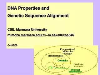
Computational. Computational. Molecular. Molecular. Biology. Biology. Bioinformatics. Bioinformatics. Genomics. Genomics. Genomics. Genomics. Functional. Functional. genomics. genomics. Proteomics. Proteomics. Structural. Structural. Structural. Structural. bioinformatics.

Computational
E N D
Presentation Transcript
Computational Computational Molecular Molecular Biology Biology Bioinformatics Bioinformatics Genomics Genomics Genomics Genomics Functional Functional genomics genomics Proteomics Proteomics Structural Structural Structural Structural bioinformatics bioinformatics bioinformatics bioinformatics DNA Properties and Genetic Sequence AlignmentCSE, Marmara University mimoza.marmara.edu.tr/~m.sakalli/cse546Oct/19/09
Sequence Alignment and Why • Global Alignment • Local Alignment • Suppose a cloned gene • If it is already in databases. Database Accession, Annotation (summary of structure), expression profile? Mutants? • Its protein characteristics? -Sub-localization -Soluble? -3D fold • Is there conserved regions?-Alignments?-Domains? • Is there similar sequences?-% identity?-Family member? • Evolutionary relationship?-Phylogenetic tree • Scoring Matrices • Alignment with Affine Gap Penalties • Applying algorithms to analyze genomics data • Applying Manhattan Tourist Problem to sequence comparison
a “mini” Global Alignment to get Local Local alignment Global alignment Local vs. Global Alignment Global Alignment Local Alignment—better alignment to find conserved segment --T—-CC-C-AGT—-TATGT-CAGGGGACACG—A-GCATGCAGA-GAC | || | || | | | ||| || | | | | |||| | AATTGCCGCC-GTCGT-T-TTCAG----CA-GTTATG—T-CAGAT--C tccCAGTTATGTCAGgggacacgagcatgcagagac |||||||||||| aattgccgccgtcgttttcagCAGTTATGTCAGatc Some genes only have small conserved regions between species of organisms Example: Homeobox genes have a short region called the homeodomain that is highly conserved between species. A global alignment would not find the homeodomain because it would try to align the ENTIRE sequence.
Find long ORFs, the longest ORFs first and putting together a set with minimal overlaps, identify the furthest upstream start codon. • A new found ORF might not contain a real gene. Compare it with a gene known from other species. • Different DNA sequences will give identical proteins (remember from the codon table). So there is large amount of redundancy in DNA sequence. • Conservation of a sequence between species strongly suggests that the sequence has a function that is being conserved by natural selection. • A protein being functional is more likely being conserved in evolutionary process than DNA.The organism’s survival depends on the protein being functional. • The protein 3-dimensional structure is even more conserved, because it is more closely related to enzyme activity than the amino acid sequence is. • Research subjects: To build 3-D structure from a DNA sequence
Sequence Comparison • Comparing ORF sequence to a database of known protein sequences from many species. • BLAST is the standard (BLAST = Basic Local Alignment Search Tool) • BLAST is based on the concept that if you compare the same (that is, homologous) protein from many different species. • - Some amino acids readily substitute for each other and some others almost are unique and never will substitute. • A substitution matrix, giving a score for each amino acid position in the proteins being compared These weights are given based on biological evidence. Alignments can be thought of as mutations in the sequence. Some of these mutations have little effect on the organism’s function, therefore some penalties, δ(vi , wj), will be less harsh than others.
Terminology: query sequence: sequence entered. Sequences matching are subject sequences. • Gene B. meg. It is 174 amino acids lon, written in “fasta” format: Starts with > and immediately followed by an identifier (ORF00135), and then some comments. And then follows the sequence. • Scoring matrices: • Scoring matrices are created based on biological evidences. • Alignments can be thought of as two sequences that differ due to mutations in the sequence. • Some of these mutations have little effect on the organism’s function, therefore some penalties, δ(vi , wj), will be less harsh than others. • Different amino acids might have a positive score. Ie due to having positively charged. • Score S is calculated by summing the scores assigned for matches, mismatches and gaps (creation/extension scores). • The scores are given by the specified substitution matrix. • PAM (Percent Accepted Mutation): for evolutionary studies. • For example in PAM1, 1 accepted point mutation per 100 amino acids is required. • BLOSUM (BLOcks amino acid SUbstitution Matrix): for finding common motifs. For example in BLOSUM62, the alignment is created using sequences sharing no more than 62% identity. • How the matrices were created: • Very similar sequences were aligned. • From these alignments, the frequency of substitution between each pair of amino acids was calculated and then PAM1 was built. • After normalizing to log-odds format, the full series of PAM matrices can be calculated by multiplying the PAM1 matrix by itself. >ORF00135 |chromosome 538197-538721 revcomp MKAKLIQYVYDAECRLFKSVNQHFDRKHLNRFLRLLTHAGGATFTIVIACLLLFLYPSSVAYACAFSLAVSHIPVAIAKKLYPRKRPYIQLKHTKVLENPLKDHSFPSGHTTAIFSLVTPLMIVYPAFAAVLLPLAVMVGISRIYLGLHYPTDVMVGLILGIFSGAVALNIFLT
- Some matrices reflect similarity: good for database searching • - Some reflect distance: good for phylogenies • - Log-odds matrices, a normalization method for matrix values: • Sij = log (qij/(pi pj))=log (qij) – log (pi) – log (pj) • Sij is the probability that two residues, i and j, are aligned by evolutionary descent and by chance. • qij are the frequencies that i and j are observed to align in sequences known to be related. • pi and pj are their frequencies of occurrence in the set of sequences. • The most widely used local similarity algorithms are: • Smith-Waterman (http://www.ebi.ac.uk/MPsrch/) • Basic Local Alignment Search and Fast Alignment, which are based on k-tuple algorithms… • Speedwise: BLAST > FASTA > Smith-Waterman (It is VERY SLOW and uses a lots of computational power • Sensitivity/statistics: • FASTA is more sensitive to variations, misses less homologues • Smith-Waterman is even more sensitive. • BLAST calculates probabilities • FASTA more accurate for DNA-DNA search then BLAST
BLAST and FASTA variants Comparison between, FASTA:a DNA query to DNA db, or a protein query to protein db FASTX:a translated DNA query to a protein database TFASTA:a protein query to a translated DNA database BLASTN:a DNA query to DNA database. BLASTP:a protein query to protein database. BLASTX:6-frame translations of DNA query to protein database. TBLASTN:a protein query to the 6-frame translations of a DNA database. TBLASTX:6-frame translations of DNA query to the 6-frame translations of a DNA database. PSI-BLAST: Performs iterative database searches. The results from each round are incorporated into a 'position specific' score matrix, which is used for further searching BLAST results
Detailed BLAST results E value:is the expectation value or probability to find by chance hits similar to your sequence. The lower the E, the more significant the score.
Mostly genes are named with the function of their protein.at some point, some related genes had their function determined through lab work: by examining the effects of mutations in the gene, by isolating and studying the protein produced by the gene, etc. • Enzymes (end in –ase), transport across the cell membrane, genetic information processing (DNA->RNA->protein), structural proteins, sporulation and germination, and more! • Many genes (maybe 1/4 of them in a typical genome) have no known function, although they are found in several different species: conserved hypothetical genes • Every new genome has some genes that are unique: no matching BLAST hits in the database. • Are they real genes? Sometimes there is evidence in the form of messenger RNA, but usually we don’t know call them hypothetical genes • “putative” means that we think we know the gene’s function but we aren’t sure. Putative should be followed by the function name.
(Basic Similarity) Homology Search, The Knuth-Morris-Pratt Algorithm (exact match) • All similarity searching methods rely on the concepts of alignment and a distance measurements between. • Associated with a similarity score calculated from a distance matrix for example the number of DNA base that are different between. • Exact String Matching • Naive brute force algorithm searching for pattern p in text t, lengths m=|p| and n=|t|, then the worst case complexity Θ(nm) . Sliding the pattern across from left to right, one step at a time, but it is possible to shift more than one, given a certain length of the pattern sought is detected in the text. Just imagine it.. • The Knuth-Morris-Pratt Algorithm - Complexity • The algorithm of KMP algorithm takes into account the information gained during previous symbol comparisons, with prefix and suffix definitions. Never re-compares a text symbol that has matched a pattern symbol. • The complexity of the searching phase is in O(n). • Its preprocessing stage (the pattern search) has a complexity of O(m). m<=n. • Therefore overall complexity is in O(n).
The Knuth-Morris-Pratt Algorithm - Definitions • Definition: Let A be an alphabet, and x be a string of length k, x=x_0, x_1, …, x_(k) over A. • A prefix of x, is a substring u, u=u_0, u_1, …,u_b, where b<k, 0<={b,k}, • A suffix of x, is a substring u, u=u_{k-b}, u_{k-b+1}, …, u_{k}, where 0<b<=k. • Called proper prefix or suffix of u, if b<k. • A border of x is a substring which appears as a proper suffix and a proper prefix of x and its length is b. • Example x=abacab. Proper Prefixes: є, a, ab, aba, abac, abaca. Proper Suffixes: є, b, ab, cab, acab, bacab. Borders: є, ab, with lengths of 0 and 2. • The empty string є is always a border of x, but itself has no border. • 0123456789... • abcabcabd • abcabd • abcabd • Matching prefix p=abcab, length 5, mismatch occurs at position 5 between c and b, the widest (border length) - of the prefix of p matching to suffix of p -, b=2, then the shift distance is |p|-|b|=5-2. • Theorem: Let r, s be borders of a string x, where |r| < |s|. Then r is a border of s. • Proof.
The Knuth-Morris-Pratt Algorithm – Preprocessing generating a look-up table • Definition: Let x be a string and aA a symbol. A border r of x can be extended by a, if ra (r appended a) is a border of xa. • j: 0123456 • p[j]: ababaa • b[j]: -1001231 • void kmpPreprocess() • { • int i=0, j=-1; • b[i] = j; • while (i<m) //O(m) length of the pattern • { //initial j=-1, i=0; j<i.. • while (j>=0 && p[i]!=p[j]) j=b[j]; //if mismatch, reduce j, max reduction until j<0 • i++; j++; //if increase with.. • b[i] = j; • } • }
The Knuth-Morris-Pratt Algorithm – Searching • void kmpSearch() • { • int i=0, j=0; • while (i<n) //Text length • { • while (j>=0 && t[i]!=p[j]) j=b[j]; //if mismatch, max reduction to –j; • i++; j++; //max j can be m, hits to a match • if (j==m) //m pattern length • { • report(i-j); • j=b[j]; • } • } • } • Example: • 0123 4567 89... • abab baba a • abab ac • ab abac • abab ac • ab ab ac • ab abac • Max number of comparisons 2n. //border length b[j] lookup j: 0123456 p[j]: ababaa b[j]: -1001231
Boyer-Moore algorithm • Starts comparison from the rightmost, and if the rightmost does not match and if not occurs in the pattern at all, then the pattern can be shifted by m. • The Boyer-Moore algorithm uses two different heuristics for determining the maximum possible shift distance in case of a mismatch: the "bad character" and the "good suffix" heuristics. Both heuristics can lead to a shift distance of m. • 0 1 2 3 4 5 6 7 8 9 ... 0 1 2 3 4 5 6 7 8 9 ... • a b b a d a b a c b a a a b a b a b a c b a • b a b a c a b b a b • b a b a c a b b a b //borders matching • Occurrence Function. occ(p, a) = max{ j | pj = a}, occ(text, x) = 2, occ(text, t) = max{0, 3}=3. • The pattern is shifted by the longest of the two distances given by the bad chrtr and the good suffix heuristics. • Left: Bad suffix character. Example of bad pattern heuristics (a special case of good suffix heuristics). Needs preprocessing, borders.. • Requires only O(n/m) comparisons, if always the first symbol mismatch occurs. • The preprocessing for the good suffix heuristics is rather difficult to understand and to implement. • Therefore, modified versions of the BM algorithm in which the good suffix heuristics are avoided. The argument is that the bad character heuristics would avoid comparisons, while good suffix heuristics would not avoid. • Bad character heuristics, - the Horspool algorithm or the Sunday algorithm suit better.
Bad-character mismatch of BM, versus Horspool Algorithm, and Sunday’s Algorithm • 0 1 2 3 4 5 6 7 8 9 ... 0 1 2 3 4 5 6 7 8 9 ... 0 1 2 3 4 5 6 7 8 9 ... • a b c a b d b a c b a a b c a b d b a c b a a b c a b d b a c b a • b c b a b b c b a b b c b a b • b c b a b b c b a b b c b a b • the rightmost position of a in p0 ... pm-2, or -1, occ(text, x) = 2, occ(text, t) = 0, occ(next, t) = -1. • Occurrence at the leftmost (last bit) is not taken into count, best case performance O(n/m) • On the Sunday’s shifts left of the d, since d does not occur in the pattern, and the comparison can be depend on the symbol probabilities, if known, then the least probable symbol in the pattern is compared first, hoping that it does not match, for the pattern be shifted. • Skip Search Algorithm searches least likely pattern!!!.. • Minimize the false positive matches. • Information theoretic approach: Repetitive subsequences (ie poly AT) has low information content, random.. • Minimum Message Length, (MML).. uses HMM (or PFSM)..
www.bioalgorithms.info\Winfried Just Next week: Aligning Two Strings Represents each row and each column with a number and a symbol of the sequence present up to a given position. For example the sequences are represented as: Alignment as a Path in the Edit Graph A T C G T A C w 0 1 2 2 3 4 5 6 7 7 A T _ G T T A T _ A T C G T _ A _ C 0 1 2 3 4 5 5 6 6 7 (0,0) , (1,1) , (2,2), (2,3), (3,4), (4,5), (5,5), (6,6), (7,6), (7,7) 1 2 3 4 5 6 7 0 v 0 A 1 T 2 G 3 T 4 T 5 A 6 T 7