Download
1 / 60
600 likes | 712 Views
Investigating nitrate movement in Ultisol under poultry litter application, assessing pollution risk using scenarios technique, and analyzing soil physical characteristics for water movement.

E N D
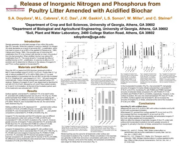
Water and Nitrate Movement in Poultry Litter Amended Soils Jaime F. Sanchez
Overall Objectives • Describe nitrate movement in an Ultisol under long term poultry litter application • Determine the physical characteristics and organic carbon content of the soil to describe the water movement in selected profiles • Determine the nitrification rates of poultry litter used in the study area • Evaluate the scenarios technique as a tool for assessment of nitrate pollution risk
N Live Oak CR 250 Poultry Farm 193 RD Suwannee County, Fl Suwannee River Basin North Florida 11,440 km2 12 counties 290,000 people SRWMD. 2000
Monitoring Area Monitoring Area Poultry Houses Poultry Houses Transect points Random points Wells
Site Characteristics • Poultry litter spread area: 11 ha • Loamy, siliceous, thermic, Arenic Paleudult • Bahia grass, Paspalum notatum • Litter production - 413 Mg y-1 • +20 years of poultry litter application • Grazed 40% of the time by 55 heads
1. Nitrate movement in soils • Describe nitrate movement in an Ultisol under long term poultry litter application • Determine soil nitrate levels in a grazed bahia pasture under a long term poultry litter application • Determine the influence of rainfall the poultry litter applications on soil and groundwater nitrate levels
1 13 2 14 15 3 4 Location and methods Nitrate: 10:1 solution in 0.01N KCl Determined with a Alpkem FlowSolution IV Autoanalyzer Weather station: established at the farm in 2001 ET: Hargreaves, 1975 and Hargreaves & Samani, 1982 Soil sampling points Wells
Nitrate changes on soil - Point 2 1 13 2 14 15 3 4 1 2 3 4 5 17Apr – 2.1 Mg 04Feb – 2.7 Mg 22Feb – 4.5 Mg 31Aug – 2.1 Mg 11Jul – 0.8 Mg
Conclusions • The levels of nitrate-N in the groundwater never exceeded the 10 mg L-1 during the study period • Although soil nitrate levels sometimes exceeded 10 mg kg-1 when amended with poultry litter at prescribed rates over the 18-month period; these peaks however, did not increase the nitrate levels over 10 mg L-1 in the groundwater • Prior management factors may be responsible for higher initial nitrate levels observed in the soils
2. Soil Characterization • Determine the soil physical characteristics and soil organic carbon to describe the water movement in selected profiles • Physical parameters determined • Bulk Density • Saturated Hydraulic Conductivity • Moisture Retention Curves • Particle Size Analysis
Soil Physical Characterization • Specific Objectives • To describe water movement through a pedo-transfer function • Verify and compare the pedo-transfer function obtained with other models of water movement
3 2 1 Location and methods Bulk Density: Cylinder method Saturated Hydraulic Conductivity: Constant head Organic Carbon: Walkley-Black Particle Size Analysis: Pipet method Water Retention Curves: Tempe Cells Soil profiles
3 0 2 10 1 20 30 40 50 60 Depth, cm 70 80 90 100 110 120 130 140 150 1.0 1.1 1.2 1.3 1.4 1.5 1.6 1.7 1.8 1.9 2.0 Bulk density, Mg m-3 Point 1 2 3 Bulk density
3 0 2 10 1 20 30 40 50 60 Depth, cm 70 80 90 100 110 120 130 140 150 0 1 2 3 4 5 6 7 8 9 10 11 12 13 14 15 Saturated Hydraulic Conductivity, cm hr-1 Point 1 2 3 Saturated Hydraulic Conductivity
3 0 2 10 1 20 30 40 50 60 Depth, cm 70 80 90 100 110 120 130 140 150 0 1 2 3 4 Organic carbon, % Point 1 2 3 Organic Carbon
3 0 2 10 1 20 30 40 50 60 Depth, cm 70 80 90 100 110 120 130 140 150 0 20 40 60 80 100 Clay, % Point 1 2 3 Clay
Water Retention Curves • Undisturbed samples • Tempe cells • Ceramic plates, ½ bar • Water column pressures • 0.3, 2.,0, 2.9, 4.4, 5.9, 7.8, 9.8, 14.7, 19.6, 33.8 kPa • Pressure Plate Extractor • 490.4 and 1471.3 kPa Retention Curves
Pedo Transfer Functions-33.8 kPa Θ33.8kPa = -1.04125 – 0.03271*C + 0.01402*M + 0.00707*CLAY + 0.03567*OC + 0.5213*BD
Pedo Transfer Functions-490.4 kPa Θ490.4kPa = -1.31440 – 0.05474*C + 0.02549*M + 0.01336*VF + 0.01143*CLAY + 0.02626*OC + 0.41434*BD
Pedo Transfer Functions-1,471.3 kPa Θ1471.3kPa = -0.71933 – 0.07436*C + 0.02.066*M + 0.00746*CLAY + 0.26567*BD
a (1 - θ / θs)1/2 (θc / θs) -b h = (1- θc / θs) 1/2 Campbell Water Retention Equation& Modifications h = a ( θ / θs) -b Campbell Where θs is water content at saturation and a and b are constants Hutson and Cass Where hcθc is the point of intersection of the exponential and parabolic curves and, hc = a [2b / (1+2b)] -b θc = 2bθs / (1+2b) The composite water retention curve is sigmoidal, continuous and has a differential water capacity of zero at saturation
0.6 0.5 0.4 Theta estimated at -33.8 kPa suction, m3 m-3 0.3 0.2 0.1 0.0 0.0 0.1 0.2 0.3 0.4 0.5 0.6 Theta observed at -33.8 kPa suction, m3 m-3 Model Campbell Pedotransfer Function Model Predictions – -33.8 kPa suction
0.6 0.5 0.4 0.3 Theta estimated at -490.4 kPa suction, m3 m-3 0.2 0.1 0.0 0.0 0.1 0.2 0.3 0.4 0.5 0.6 Theta observed at -490.4 kPa suction, m3 m-3 Model Campbell Pedotransfer Function Model Predictions – -490.4 kPa suction
0.6 0.5 0.4 Theta estimated at -1471.3 kPa suction, m3 m-3 0.3 0.2 0.1 0.0 0.0 0.1 0.2 0.3 0.4 0.5 0.6 Theta observed at -1471.3 kPa suction, m3 m-3 Model Campbell Pedotransfer Function Model Predictions – -1,471.3 kPa suction
Conclusions • The soil water retention increased as the clay content increased with depth • With some exception, water retention and bulk density were well correlated • The Campbell model better predicted the water content at different suctions compared to the PTF
3. Nitrification of Poultry Litter • Determine the nitrification rates of poultry litter used in the study area • Procedure • 450 gr of soil • 7 rates of poultry litter application (0,3,6,9,12,15,18 and 21 Mg ha-1) • Incubated at 40 ºC • Sampling at 0,1,2,3,5,7,10,15,20,30,45 and 60 days after application • N pool and first order rate constant • Nm = No [1 – e (-kt)]
N Mineralized 300 250 200 Total mineralized N (mg kg-1) 150 100 50 0 0 10 20 30 40 50 60 Incubation Time (Days) 0 1 2 3 Poultry Litter (gr) 4 5 6 7
% N Mineralized of N applied 80 60 40 % mineralizaed of N applied 20 0 0 10 20 30 40 50 60 Incubation Time (Days) Poultry Litter (gr) 1 2 3 4 5 6 7
Conclusions • Higher applications of poultry litter yielded higher levels of mineralized N • After 60 days of incubation, the net N mineralized was 61 mg kg-1 when the litter application rate was 3 Mg ha-1; the net mineralized N increased to 167 mg kg-1 when the rate of litter application was increased to 21 Mg ha-1 • 38% of the nitrogen was mineralized when 21 Mg ha-1 of poultry litter was applied vs 68% mineralized when 3 Mg ha-1 litter was applied
4. Scenarios Technique • Each scenario or coherent series of assumptions expressed in figures (numbers, tables, illustrations) -Godet, 1987 • Suggested name - Exploratory Prospective Analysis - defined as “a panorama of possible futures, or scenarios, which are not improbable in the light of past causalities, and the interaction between the intentions of interested parties”
Objectives • Evaluate the scenarios technique as a tool for assessment of nitrate pollution risk • Scenarios based on: • Water retention characteristics • Weather time series
Leachn - Hutson and Wagenet, 1992 • Richard’s equation to predict soil water dynamics • Simulate the N cycle according to Johnson et.al., 1987 • Humification process is simulated, allowing for reorganization of mineral nitrogen and CO2 losses • Ammonia pool is subjected to nitrification, volatilization and leaching and the nitrate pool is subjected to denitrification and leaching
Climatic variables • Mayo station • 30º 03’ N • 83º 11’ W • A time series of 50 years 1950-1999 • Rainfall • Maximum and minimum temperature
Best Management Practices • Application of manure between end of March and beginning of September • Application of fresh poultry manure to cover nitrogen Bahia grass, Paspalum notatum requirements • No extra inorganic fertilizers • Grazing, 40% of the time
Leachn parameters – soil physical characteristics • Water retention curves Determined • Campbell parameters Derived • Saturated hydraulic conductivity Determined • Particle size analysis Determined
Weather – Mayo Fl, 1950-1999 0 60 2 55 4 50 6 45 8 40 10 35 24H Rainfall, mm 12 30 Temperature C 14 25 16 20 18 15 20 10 22 5 24 0 0 30 60 90 120 150 180 210 240 270 300 330 360 Day of the Year
Depth=5 Depth=45 10 10 9 9 8 8 7 7 6 6 Soil nitrate, mg kg-1 Soil nitrate, mg kg-1 5 5 4 4 3 3 2 2 1 1 0 0 01SEP02 01NOV02 01JAN03 01MAR03 01MAY03 01JUL03 01SEP03 01NOV03 01SEP02 01NOV02 01JAN03 01MAR03 01MAY03 01JUL03 01SEP03 01NOV03 Date Date PLOT Observed Predicted PLOT Observed Predicted Depth=105 Depth=145 10 10 9 9 8 8 7 7 6 6 Soil nitrate, mg kg-1 Soil nitrate, mg kg-1 5 5 4 4 3 3 2 2 1 1 0 0 01SEP02 01NOV02 01JAN03 01MAR03 01MAY03 01JUL03 01SEP03 01NOV03 01SEP02 01NOV02 01JAN03 01MAR03 01MAY03 01JUL03 01SEP03 01NOV03 Date Date PLOT Observed Predicted PLOT Observed Predicted Soil Nitrate - Validation
Scenarios SCENARIO 1IFAS BMP: 50 kg ha-1 N 100 kg ha-1 N 160 kg ha-1 N SCENARIO 2IFAS BMP + 50 kg ha-1 Ammonium Nitrate SCENARIO 3IFAS BMP on SAND PROFILE SCENARIO 4IFAS BMP on Wet-Dry Sequence of years
5000 4000 3000 Nitrate in drainage, kg ha-1 2000 1000 0 0 10 20 30 40 50 Year of simulation Scenario 50N 100N 160N Scenario 1 – IFAS BMPs
Scenario 1 – IFAS BMPs 100 kg ha-1 year-1 N 145 110 75 Depth, cm 40 5 0 4.07 2.71 Nitrate mg kg-1 1.36 0.00 49 42 35 28 21 14 7 Year
Scenario 2 – IFAS BMPs + 50 kg ha-1 Ammonium nitrate 9000 8000 7000 6000 5000 Nitrate in drainage, kg ha-1 4000 3000 2000 1000 0 0 10 20 30 40 50 Year of simulation Scenario 50N 100N 160N 50F 100F 160F
Scenario 2 – IFAS BMPs + 50 kg ha-1 Ammonium nitrate 100 kg ha-1 year-1 N 9.94 6.63 Nitrate mg kg-1 3.31 145 110 75 0.00 49 Depth, cm 42 40 35 28 21 14 7 5 0 Year
Scenario 3 – IFAS BMPs - Sand Profile 6000 5500 5000 4500 4000 3500 Nitrate in drainage, kg ha-1 3000 2500 2000 1500 1000 500 0 0 10 20 30 40 50 Year of simulation Scenario 100N 160N 50S 100S 160S 50N
Scenario 3 – IFAS BMPs - Sand Profile 100 kg ha-1 year-1 N 4.28 2.85 Nitrate mg kg-1 1.43 145 110 75 Depth, cm 0.00 49 42 40 35 28 21 14 7 5 0 Year