Download
1 / 69
690 likes | 711 Views
Learn about simulating HRTFs for realistic 3D audio environments, including azimuth, elevation, ITD, IID, and HRTF calculations using computational methods.

E N D
Computer Simulation of the Head-Related Transfer Function COMP 768 Class Presentation AlokMeshram
Overview • Overview of a 3d Sound System • Head Related Transfer Functions • The Acoustic Wave Equation • Numerical Methods for Acoustic Simulation • Finite Element Method • Boundary Element Method • Finite Difference Time Domain Method • HRTF Calculation using Numerical Methods
3d Sound Systems: An Overview • 3d Sound Systems simulate auditory images • This imagery must be 3-dimensional in order to accurately simulate real world environments • This is because human listeners can perceive spatial information such as location and size • Also, the shape and size of the listener’s surroundings also affects the sound they receive
A representation of an auditory scene with relevant parameters labeled
3d Sound Systems • From the listener’s perspective, the important attributes of an auditory scene are: • Sound source positions (Azimuth, Elevation) • Sound source size and distance • The environmental context (Reverberation) • In order to simplify things, we begin with sound sources in free space (no environmental context) • Also, we will focus only on azimuth and elevation • Environment and distance can be added later
3d Sound: Azimuth and Elevation • The sounds received at the ears change as the azimuth and the elevation of the source change • The difference between the signals received at the two ears are characterized by: • The Interaural Time Difference (ITD) • The Interaural Intensity Difference (IID) • Lord Rayleigh calculated these for a spherical head in his “Duplex Theory” (1907)
3d Sound: Azimuth and Elevation Left: Sound reaches the two ears at different times (ITD) Right: The Head’s “shadow” causes the intensity of the sound at one ear to be lower than the other (IID)
3d Sound: Azimuth and Elevation • However, ITD and IID values cannot be used to uniquely determine a source’s location For a spherical head, points lying on the “Cone of Confusion” have the same ITD and IID values
Head Related Transfer Functions • ITDs and IIDs don’t account for an important part of the human auditory system: outer ears • The outer ears (pinnae) change incoming sound depending on the source’s azimuth and elevation • Like the ITD and the IID, this filtering is a cue that our auditory system uses for localization • The Head Related Transfer Function (HRTF) encodes all of these changes
Head Related Transfer Functions • The Head Related Transfer Function for each ear can be defined as: • Where: • ω represents frequency and θ,φ represent elevation and azimuth respectively • HL(ω,θ,φ) and HR(ω,θ,φ) are the left and right HRTFs • XL(ω) and XR(ω) are the Fourier Transforms of the signals received by the Left and the Right ears • X(ω) is the Fourier Transform of the source signal
Head Related Transfer Functions • HRTFs are key components of 3d Sound Systems • This is because HRTFs can be used to obtain the signals received at the listener’s ears given a sound source and its location (using convolution) • This is simple to implement and is fast as it involves simple operations (convolution) • Thus, without much cost, an HRTF based system adds location information to sound
Head Related Transfer Functions • HRTFs are complicated functions that depend strongly on head and ear geometry, differing from person to person HRTF data for 3 different people for the same source location
Head Related Transfer Functions • Researchers obtain HRTFs through physical measurements. This is slow and expensive. • On the other hand, commercial 3d Sound systems use simple HRTF models or measurements made on dummy heads • However, best results are obtained when the listener’s own HRTF is used. Hence there has been some focus on using computational methods to simulate HRTFs
Head Related Transfer Functions • Computer simulation of HRTFs use head geometry and material parameters as input • They simulate the propagation of sound around and through the head from the source (an impulse) located at various positions • The signals at the ears are Impulse Responses (HRIRs) through which we obtain the HRTFs • We’ll review some sound simulation methods to understand this better
The Acoustic Wave Equation • We will begin with the 1D case and extend it. Newton’s Second Law is: • Dividing both sides by Volume, we get : • We can rewrite it in terms of Pressure Gradient: • The negative sign accounts for the fact that Force due to a Pressure Gradient is in the direction of decreasing Pressure.
The Acoustic Wave Equation • Next, consider a small section (length Δx) of a tube (cross section A). This tube is filled with a material that has Bulk Modulus B defined as: • The Volume of the small section is: • Due to a disturbance the particles of the material move from their original position by a position dependent amount s(x). The change in Volume is:
The Acoustic Wave Equation • Substituting this in the Bulk Modulus equation: • Differentiating with respect to time, we get: • This is known as the continuity equation, and besides Newton’s law it establishes another relation between Pressure and particle velocity
The Acoustic Wave Equation • Differentiating Newton’s Law w.r.t position: • Differentiating Continuity Equation w.r.t time: • Combining, we get the Acoustic Wave Equation:
The Acoustic Wave Equation • Extension to 3d is simple. We use gradients and divergence instead of spatial derivatives: • Note that v is a vector here (it’s in bold). As before, we get the Acoustic Wave Equation by combining these two equations: • Where is the Laplacian
The Acoustic Wave Equation • Among the solutions to the Acoustic Wave Equation, of particular interest are those with sinusoidal time dependence: • Substituting this in the Acoustic Wave Equation: • This is also known as the Helmholtz equation.
Numerical Methods for Acoustic Simulation • We’ve studied Numerical Methods used for integrating Ordinary Differential Equations • However, the Wave Equation is a Partial Differential Equation in space and time • Here we’ll review some numerical methods used to obtain solutions for PDEs like the Wave Equation: • Here f(x,t) represents sound sources
Finite Element Method • The general Finite Element Method(FEM) is quite complicated and involves concepts such as Hilbert and Solobev Spaces • Here, we’ll develop a simpler version from basics • The method we’ll develop will be specifically for the acoustic wave equation • We’ll begin by looking at an overview of the general strategy of the method
Finite Element Method: Overview • An important point: the Acoustic Wave Equation is a PDE in space and time • This means that its solution must be calculated for spatially as well as across time • The FEM’s strategy is to use basis functions distributed spatially over the region of interest • Each of these basis functions is associated with a time-dependent coefficient
Finite Element Method: Overview • The overall solution is the sum of the basis functions weighted by their time dependent coefficients • The advantage of using this strategy is that we can use mathematical manipulation to reduce the time-and-space dependent PDE to a set of time-dependent ODEs • These ODEs can be solved using conventional integrators such as RK4 or the Implicit methods to get the full solution
Finite Element Method: Overview Top: “Hat” basis functions in [0,1] used to divide 1-dimensional space. Notice their overlap and their sum for some coefficients (in red). Left: Pyramidal basis functions over a triangulation of a 2D region
Finite Element Method • We now discuss the actual formulation of the FEM for the acoustic equation. We start with the following representation of the solution: • Next, we consider the Acoustic Wave Equation:
Finite Element Method • Let V be the set of bounded, continuous functions defined on Ω having piecewise continuous first derivatives and fulfilling the spatial boundary conditions of the problem, and let v be its element • Then using the fundamental theorem of calculus of variations and the wave equation, we have: • Using Gauss’ Divergence Theorem:
Finite Element Method • Substituting our approximation of P(t,x) into this equation, we get (after much mathematical manipulation):
Finite Element Method • We can represent the previous equation as a Matrix equation solving N simultaneous equations (one for each basis function): • Where,
Finite Element Method • As mentioned earlier, we have now reduced the Wave Equation to a system of N simultaneous time-dependent ODEs that can be solved by using regular integration methods • This will give us the individual (t) that we need along with the basis functions to represent the full solution
Boundary Element Method Overview • Instead of discretizing all space (as in FEM), the Boundary Element Method (BEM) works on the discretization of a boundary (surface) in space • To be able to apply BEM, one must reformulate the problem as a Boundary Integral equation • Often, this requires some analytical calculation • Hence BEM can be said to be halfway between analytical methods and numerical methods
Boundary Element Method Overview • We’ll assume sinusoidal time dependence for our solution of the wave equation • We get the Helmholtz equation as a result • It is converted into boundary integrals using either the “direct” or the “indirect” method • To get the solution on the boundary, we use FEM on the boundary mesh. The boundary solution can then be used to get the full solution.
Boundary Element Method • We start with the wave equation: • As mentioned earlier, when we assume sinusoidal time dependence, we get: • Where u(x) is a complex valued function called the complex acoustic pressure • It’s magnitude and argument determines the magnitude and phase of the pressure wave at x
Boundary Element Method • With sinusoidal time dependence, the wave equation reduces to the Helmholtz equation: • We can convert this PDE into a boundary integral equation using the impedance boundary condition: • Here, g is 0 for a scattering problem (which we are interested in) and β(x) is the material dependent relative surface admittance of the scattering surface (usually constant)
Boundary Element Method • We convert the Helmholtz equation into an integral equation by using its analytical solution for a point source in free space • For a point source at x0, the solution at x is given by the free-field Green function: • We also use Green’s Second Theorem:
Boundary Element Method • We treat x and x0 as constants and use y as the variable in our integral equations. We choose: • Note that u(y) is the unknown solution we’re looking for and G(y,x) is the acoustic pressure at y due to a point in x. Since both of these satisfy the Helmholtz equation, we use Green’s Second Theorem to get:
Boundary Element Method • Note that u(y) and G(y,x) are singular at x0 and x respectively. Also, we’re trying to solve the problem within a bounded region D. • Using these considerations, we get (in the limit of almost including x and x0 in D) : • Now we make use of the impedance boundary condition that we had:
Boundary Element Method • After substituting the boundary condition we get our first boundary integral equation that relates the solution to its values on the boundary (this equation is not valid on the boundary): • When x is on the boundary, we get a second boundary integral equation (if the boundary is smooth, i.e, without corners):
Boundary Element Method • We use the BEM to solve the second equation, giving us values for u(x) on the boundary • This can be used with the first equation to obtain values for all space inside the bounded region D • This was the formulation of the “interior problem” where the boundary scatters sound due to sources inside it • It can be extended for the “exterior problem”
Boundary Element Method • In BEM we solve the boundary integral formulation of the problem using FEM • We subdivide the boundary into N smooth pieces, γ1,….,γN • On each of these pieces, we assume a representation for u(x) (usually polynomial) • As an example, we’ll assume that u(x) has a constant value uj on the jth piece
Boundary Element Method • With this approximation, the first boundary integral equation (points not on the boundary) is: • And the second boundary integral equation (for points on the boundary) is: • To solve for the uj’s, we use the collocation method: we assume that the second equation holds exactly for the centroidxi of each piece
Boundary Element Method • With this approximation, the second equation is: • Or, equivalently: • Where: • u is a column vector consisting of uj’s • b is a column vector with ith entry = G(x0,xi) • And B is a matrix with:
Boundary Element Method • By solving this equation for u, we get uj for each of the pieces on the boundary • This could be used to solve the first boundary integral equation to get the values of u(x) for all space • Note that the integrals over γj could also be approximated. This would make the solution simpler and faster, but less accurate
Boundary Element Method • We changed the Helmholtz equation to Boundary Integral Equations using the “direct method” • The “indirect method” uses functions called the single-layer and double layer potentials. These and their normal derivatives have “jumps” on and across the boundary • These are expressed in boundary integral form and are automatically solutions of the Helmholtz equation. We then try to express the problem and its boundary condition in their terms
Finite Difference Time Domain • The Finite Difference Time Domain (FDTD) method was originally developed for Electromagnetic problems, but is also applicable to Acoustic problems • It represents relevant differentials in the PDE as Finite Differences • Unlike the BEM that we considered, FDTD is a Time Domain method, meaning that it iterates over time
Finite Difference Time Domain • FDTD approximates both spatial and temporal derivatives by finite differences. Consider the Taylor series expansion of a function f(x) about the point x0 with an offset of ±δ/2 : • Subtracting: • Dividing by δ and rearranging, we get:
Finite Difference Time Domain • Ignoring the O(δ2) term, this is a finite difference approximation of the derivate • We’ll begin with the 1-d FDTD for simplicity. Consider the equations that resulted in the wave equation: • We’ll replace the derivatives in this equation with finite differences
Finite Difference Time Domain • In order to use finite differences, we’ll need to discretize time and space in the following way: • We’ll represent space by points spread Δx apart • We’ll represent time by points spread Δt apart • We’ll use a staggered grid over space and time • This allows us to alternate iterations over P and v and hence calculate both over space and time
Finite Difference Time Domain The staggered grid over space and time used in the FDTD method
Finite Difference Time Domain • With this staggered grid, at ((i+1/2)Δx, nΔt), using finite differences we get our first update equation • This essentially updates the value of v at a future time based on its current value and the current value of P at two neighbouring spatial positions