Download
1 / 64
640 likes | 661 Views
Explore how modern evolutionary political economy combines Veblenian rejection of statics with Schumpeterian model of transformational growth, addressing the incompatibility of static and dynamic reasoning. Dynamically analyze supply and demand in a market to understand the limitations of static models. Learn about the importance of stable equilibria and non-linear functions in creating realistic economic models.

E N D
Advanced Political Economy Complexity & self-organisation
Recap • Veblen & Schumpeter: two different directions for evolutionary economics • Veblen: anti-neoclassical • statics must be abandoned; • but no model • Schumpeter: pro-neoclassical • statics can co-exist with disequilibrium transformational growth; • a model • Modern evolutionary political economy combines V&B: • Veblenian rejection of (neoclassical) statics • Schumpeterian model of transformational growth
Why the hybrid? • Incompatibility of static & dynamic/evolutionary reasoning • Neoclassical economists tend to think: • “Evolution leads to optimising behaviour” • “Dynamics explains movement from one equilibrium point to another” • So “statics is long run dynamics” • also believed by Sraffian economists • implicit in Post Keynesian or Marxian analysis using comparative static or simultaneous equation methods Statics Dynamics Evolution
Why the hybrid? • Modern mathematics reverses this • Field of evolution larger than dynamics • Dynamics larger than statics • Results of evolutionary analysis more general than dynamics • But two generally consistent • Results of dynamics more general than statics • & GENERALLY INCONSISTENT • Dynamic results correct if actual system dynamic/evolutionary Evolution Dynamics Statics • An example: supply and demand analysis
Supply & Demand Analysis • Typical supply & demand exercise: • Demand a decreasing linear function of quantity • Supply an increasing linear function of quantity • Equate the two to find equilibrium Q & P: • Two equations return same result…
Supply & Demand Analysis • An example: • D(Q)=1000-2/10000000 Q • S(Q)=-100+1/10000000 Q
Supply & Demand Analysis • “X” marks the spot! • (Are neoclassical economists really just frustrated pirates?…)
Supply & Demand Analysis • What if initial price isn’t equilibrium price; how does it get there? • Dynamic analysis • Demand price and supply price as functions of time • Producers plan output based on last year’s prices • Consumers react to today’s prices • Convergence to equilibrium over time…
Supply & Demand Analysis • Confirming that this gives the same result as static analysis • Try with initial quantity 10% more than Qe:
Supply & Demand Analysis • Convergence • So “Statics is long run dynamics”? • Let’s try another demand & supply pair…
Supply & Demand Analysis • D(Q)=1000+5/100000000 Q • S(Q)=-100+1/10000000 Q • Meaningful (non-negative) equilibrium price & quantity as before • The dynamic answer…?
Dynamic Instability • Whoops! • Quantity unstable • Cause: slope of supply curve steeper than demand • But also unrealistic: negative quantities • Dynamic model must be wrong then?…
Dynamic Instability • Model of single Market • Converges to equilibrium if b>d • Consumers’ more responsive than suppliers • Diverges from equilibrium if b<d • Suppliers more responsive than consumers • Two possibilities • Either consumers are more volatile than suppliers • Contradicted by the data • Or the model is wrong somehow… • Similar debate occurred in IS-LM modelling:
Dynamic Instability • Hicks (father of IS-LM analysis) on instability • Harrod “welcomes the instability of his system, because he believes it to be an explanation of the tendency to fluctuation which exists in the real world. I think, as I shall proceed to show, that something of this sort may well have much to do with the tendency to fluctuation. But mathematical instability does not in itself elucidate fluctuation. A mathematically unstable system does not fluctuate; it just breaks down. The unstable position is one in which it will not tend to remain.” (Hicks 1949) • I.e., “models must have stable equilibria”
Dynamic Instability • Kaldor analysed dynamics of IS-LM model • Stable if “slope of S”> “slope of I” • “any disturbances … would be followed by the re-establishment of a new equilibrium, … this … assumes more stability than the real world, in fact, appears to possess.” (80) • Unstable if “slope of I”> “slope of S” • “the economic system would always be rushing either towards a state of hyper-inflation … or towards total collapse… this possibility can be dismissed” (80) • “Since thus neither of these two assumptions can be justified, we are left with the conclusion that the I and S functions cannot both be linear.” (81) • I.e. “models must have nonlinear functions”
Dynamic Instability • 1st set of insights not known to Schumpeter • Simple (non-evolutionary) models of market can fail to converge to equilibrium under realistic conditions (suppliers more responsive than consumers, investors more responsive than savers) • Models can have unstable dynamics and not break down if functions nonlinear • Underlying static partial equilibrium model need not converge to equilibrium… • What about general equilibrium? • 2nd insight not known to Schumeter (or many economists today!) • General “equilibrium” is unstable
Dynamic Instability • Schumpeter’s faith in equilibrium tendency of non-evolutionary markets derived from Walras • Walras believed market system would find equilibrium prices and quantities by“tatonnement” (“groping”) process • Start with randomly chosen starting point • Adjust prices iteratively • Increase price where demand > supply • Decrease price where demand < supply • Converge to equilibrium prices & quantities • In Walras’ words…
Dynamic Instability • “Once the prices … have been cried at random…, each party … will offer … those goods or services of which he thinks he has relatively too much, and he will demand those articles of which he thinks he has relatively too little … the prices of those things for which the demand exceeds the offer will rise, and the prices of those things of which the offer exceeds the demand will fall. New prices now having been cried, each party to the exchange will offer and demand new quantities. And again prices will rise or fall until the demand and the offer of each good and each service are equal…” (Walras 1874) • Convergence to general equilibrium over time?
Walras’ General Equilibrium: the Problem • “This will appear probable if we remember that the change from p’b to p’’b, which reduced the above inequality to an equality, exerted a direct influence that was invariably in the direction of equality at least so far as the demand for (B) was concerned; while the [consequent] changes from p’c to p’’c, p’d to p’’d, …, which moved the foregoing inequality farther away from equality, exerted indirect influences, some in the direction of equality and some in the opposite direction, at least so far as the demand for (B) was concerned, so that up to a certain point they cancelled each other out. Hence, the new system of prices (p’’b, p’’c, p’’d, …) is closer to equilibrium than the old system of prices (p’b, p’c, p’d, …); and it is only necessary to continue this process along the same lines for the system to move closer and closer to equilibrium.” (Walras 1874 [1954]:; my emphasis)
General Disequilibrium • General equilibrium requires stable output & prices • Yt= Yt-1 = Ye (or with growth) Yt= (1+g) Yt-1 • Where Y = vector of all commodities in economy • Pt = Pt-1 = Pe • Where P = vector of relative prices of all commodities in economy • Constant relative prices • Modern maths shows these two inconsistent… • Either prices stable & quantities unstable, or • prices unstable & quantities stable • But not both (Jorgenson ‘60,61; McManus ‘63, Blatt ’83) • Consider simplest possible “GE” system…
Can General Equilibrium be in equilibrium? • Simplest possible “real world” model • n markets • Commodities produced using input-output system • Spot markets for sale of output (“supply=demand”) • All output in year t becomes input in year t+1 • Consumption “internalised” • Economy growing over time • For equilibrium, • Outputs in year 0 must be sufficient for production in year 1 • Prices must enable producers to buy all inputs • Conditions expressed in matrix equations:
Can General Equilibrium be in equilibrium? • Outputs in year t+1 “output input” transformation of inputs in previous period t: Outputs in 2004 areinputs for 2005 Production process derived from “productive” input-output matrix Output in 2005(vector of outputs) • For stable growth, each sector must grow at the same rate (a % p.a.) 2005’s output of socks,DVD players, etc., is a%greater than 2004’s
Can General Equilibrium be in equilibrium? • Two conditions on production can be combined using matrix maths… The production relation… Has to equal growth condition… Equating them… Rearrange using matrix rules… I is matrix equivalent of 1… So this bit has to be somehow equivalent to zero for this equation to be feasible
Can General Equilibrium be in equilibrium? is equivalent to zero if • The expression its “determinant” is equal to zero; more on that soon • Price condition also expressed in matrix equation • Prices must enable producers to purchase necessary inputs • For equilibrium, relative prices must be constant (p) • Cost of inputs is p (list of prices) times A (table of outputs produced from inputs) times equilibrium rate of profit p: Table of outputsproduced frominputs List of prices Uniform profit rate
Can General Equilibrium be in equilibrium? • Rearrange using matrix rules • Order of multiplication important: • (1) Multiply both sides by inverse of A • (2) A times its inverse equals I (matrix with 1’s on diagonal & 0’s elsewhere) • (3) Move to LHS: • (4) Group on p:
Can General Equilibrium be in equilibrium? is equivalent to zero if • The expression its “determinant” is equal to zero… • Matrices have a property called “eigenvalues” • Basically, roots (zeroes) of polynomial—where it crosses x-axis • (1 root for y=a+bx, 2 for y=a+bx+cx2, etc.) • For stability, biggest root must be less than 1 • Problem: A & A-1 have inverse roots… • If ½ biggest “eigenvalue” of A, then 2 is biggest eigenvalue of A-1. • Not a problem if all eigenvalues of A < 0 • -½ and -2 both less than zero • Unfortunately…
Can General Equilibrium be in equilibrium? • Matrix A derived from table of inputs needed to produce outputs • Input-output table has all non-negative entries • Can’t use negative quantities of commodity as input • Advanced maths theorems (“Perron-Frobenius”) show that A’s biggest eigenvalue must be > 0 • So either A or A-1 (or both) must have root > 1 • If A has root of ½ then A-1 has root of 2 • Results: • Either prices or quantities must be unstable • If system diverges a fraction from stability, it will never return… • “General Equilibrium” will never be in equilibrium…
Can General Equilibrium be in equilibrium? • Intuition: • Walras hoped “direct effects” of price changes • Banana supply exceeds demand banana price falls closer to equilibrium • would outweigh “indirect effects” • Banana price fall fall in income for banana producers fall in demand for biscuits feedback on banana industry… • Maths shows not the case: plausible model of growing production economy unstable; feedback effects outweigh direct
Can General Equilibrium be in equilibrium? • Neoclassical reactions? • (1) “It’s just an artefact of matrices” • (2) “Let’s find ways to make it stable!” • (3) “Let’s ignore stability” • (1) “It’s just an artefact of matrices” • Input-output table strictly linear: has rigid proportions between inputs (commodities) & outputs • Neoclassical production functions nonlinear: variable proportions, input substitution (labor for capital…) • Therefore neoclassical model will be stable while IO/matrix/Leontief systems will not… Wrong!
“It’s just an artefact of matrices” • Matrix is linear • like b in y(x)=a+bx only with many variables • Neoclassical production functions are nonlinear • like y(x)=a+bx+cx2+dx3+… • But • Any nonlinear function can be approximated by polynomial • E.g., sin(x): • “Linear bit” of sin(x) is x • Best guess for sin(x) near x=0 is x • “Linear bit” of production function is IO matrix • Stability near equilibrium determined by linear bit only
“It’s just an artefact of matrices” • Linear part “rules the roost” the closer you get to equilibrium • Linear bit of any nonlinear production function is IO matrix • Its stability determines system stability near equilibrium: nonlinear bits irrelevant
“It’s just an artefact of matrices” • Nonlinear “production function” might stop prices/quantities becoming crazy • Negative prices or quantities… • But won’t make equilibrium stable • Multiple “supply & demand” markets can’t all be in equilibrium • unless started out there and never disturbed… • which takes us to (2) “Let’s find ways to make it stable!” • First neoclassical to realise instability problem was Jorgenson (1960)…
(2) “Let’s find ways to make it stable!” • “If the output system is relatively stable, the price system cannot be, and vice versa… ” (Jorgenson 1960: 895) • “The conclusion is that excess capacity (or positive profit levels or both) is necessary … for the interpretation of the dynamic input-output system … as a model of an actual economy…” (Jorgenson 1960: 893) • So far so good; but then in 1961… • “To avoid dual instability, a number of re-interpretations of the basic model have been proposed… In this paper, a third re-interpretation … is suggested…” (Jorgenson 1961: 106)
(2) “Let’s find ways to make it stable!” • “First, the behavior of the system depends not only on the technological characteristics of the system, but also on the behavior of economic decision-makers in each of the sectors of the economy. Secondly, the complete system surmounts the difficulties associated with dual instability; by suitable restrictions on the initial values of the disequilibrium variables, the non-negativity of all economic variables is preserved…” • Introduced stocks & Reserve Bank interest rate to try to stabilise model; • Got maths wrong! (See Blatt 1983: 134, Jorgenson 1961: 112, 115) System still unstable… • Other equally flawed attempts (turnpike theorems etc.); so…
(3) “Let’s ignore stability” • Dominant model of general equilibrium “Arrow-Debreu” • “Model” designed to remove dynamics entirely • “For any economic agent a complete action plan (made now for the whole future)…” • No time process: • “Market” occurs once only in history of planet • All transactions for all time take place at once • Uncertainty re “future” abolished: • “A contract for the transfer of a commodity now specifies, … an event on the occurrence of which the transfer is conditional. This new definition of a commodity allows one to obtain a theory of uncertainty … formally identical with the theory of certainty developed in the preceding chapters.”
General Disequilibrium • ‘There exist known systems, therefore, in which the important and interesting features of the system are “essentially dynamic”, in the sense that they are not just small perturbations around some equilibrium state, perturbations which can be understood by starting from a study of the equilibrium state and tacking on the dynamics as an afterthought.’ • ‘If it should be true that a competitive market system is of this kind, then… No progress can then be made by continuing along the road that economists have been following for 200 years. The study of economic equilibrium is then little more than a waste of time and effort…’ Blatt (1983: 5-6)
General Dynamics • Schumpeter’s evolutionary economics was done by “starting from a study of the equilibrium state and tacking on evolution as an afterthought” • We now know this can’t be done • So modern evolutionary economics • Veblenian anti-equilibrium, Schumpeterian models • Builds dynamic models & add evolution later; or • Builds evolutionary models from the outset • Former approach more common • Easier (potentially dangerous reason!) • Can incorporate “vision” of given economic theory (Marx, Keynes,…) • Close match to slowly evolving systems • Insights from complex systems to evolution
In summary… • Summarising validity of analytic techniques & relations between them: • Now insights on evolution from complex systems…
Complexity & Evolution… • Previous supply & demand model “linear” • Variables added together • Only variables and constants • Kaldor’s insight—real world cannot be this simple • Variables must interact in more complex ways than simple addition • Models with nonlinear relations between variables generate complex behaviour from even “simple” models • Two examples • Discrete logistic model of population • Lorenz’s “quasi-quadratic” weather model
Complexity & Evolution… • Logistic population model • Simplest population model is: • This year’s population • Equals last year’s • Multiplied by growth rate • Model predicts population grows to infinity • But real-world populations will hit constraints • Simplest constraint • Cow tramples grass another cow could have eaten • Interaction reduces life expectancy • Interaction function of number of animals squared:
Complexity & Evolution… • Ratio a/b gives “equilibrium” population • For b=0, exponential growth of population forever:
Complexity & Evolution… • For b>0, population first rises at accelerating rate and then slowly tapers to equilibrium level:
Complexity & Evolution… • For a=2 (2 births per animal per cycle), a “2-cycle” results • Population overshoots carrying capacity • Interactions reduce population to below carrying capacity • And so on forever…
Complexity & Evolution… • For a>2.7, chaos • Population bounces around in unpredictable way • Cycles never quite repeat (aperiodic) but never cease either • But behind the apparent disorder, structure—hence “complexity” rather than “chaos” theory
Complexity & Evolution… • Another example: Lorenz’s weather model: simple system 3 equations, 3 unknowns, 3 constants… • Just 2 semi-quadratic nonlinear terms z.x and x.y x displacement y displacement temperature gradient • Model has 3 equilibria • All 3 are unstable • Generates incredibly complex cycles that are • Highly sensitive to initial conditions; but • Have underlying common structure
Complexity & Evolution… • x,y,z values bounce around like crazy…
Complexity & Evolution… • Small change in initial conditions has huge impact on eventual system path
Complexity & Evolution… • Behind the apparent chaos, an incredibly intricate structure… • Basic feature: system never even approaches equilibria Equilibrium 2 Equilibrium 1 Equilibrium 3
Complexity & Evolution… • Equilibrium highly unstable: start just next to it and get propelled away instantly… • Strange role of equilibria in nonlinear dynamics/evolution… Start near equilibrium 3
Complexity & Evolution… • Systems almost always have unstable equilibria • Many technical ways to measure degree of stability of dynamic system • Dominant eigenvalue, Lyupanov exponent, Hurst exponent,… • Basic idea of all measures: • Greater than one value, system diverges from equilibrium (eigenvalue) • Greater than another, initial starting points spread apart in time—“sensitive dependence on initial conditions”, “butterfly effect” • Greater than another, system inherently unstable: fluctuations not only due to random shocks but also inherent instability of system feedbacks