Neuron PRM: A Framework for Constructing Cortical Networks
220 likes | 381 Views
By Pavan kumar V.V.N. Neuron PRM: A Framework for Constructing Cortical Networks. Introduction. Brain’s has extraordinary computational power which is determined in large part by the topology and geometry of its structures.

Neuron PRM: A Framework for Constructing Cortical Networks
E N D
Presentation Transcript
By Pavan kumar V.V.N Neuron PRM: A Framework for Constructing Cortical Networks
Introduction • Brain’s has extraordinary computational power which is determined in large part by the topology and geometry of its structures. • Brain Tissue Scanner (BTS) is the unique instrument which will enable an entire mouse brain to be imaged and reconstructed at the neuronal level of detail.
Introduction • BTS will take approximately one month to scan the entire mouse brain • Since only a small percentage(less than 10%) of neurons will be stained, the neurons reconstructed from BTS data will be augmented with synthetic neurons that are grown based on the measured biological neurons.
Introduction • In this paper generation and connection of the anatomically realistic synthetic neurons is explained. • Strategy used is probabilistic roadmap methods(PRM) • In PRM nodes represent neurons and edges represent connections(synapses).
Neuron PRM Framework • Goal is to map and understand the connectivity and geometry of the cortical network. • The cerebral cortex is partitioned into a set of finite elements (FEs). • Then there are two stages 1.Neuron generation 2.Synapses generation The basic building blocks of this process are below.
Neuron PRM Framework: Finiteelements, Neuron generation/connection, roadmap graph, and database
Generation of Neurons • An abstract neuroncontains information regarding position, type, associated FE, and a unique ID. • Position and type are generated randomly based on some given statistical distribution stored in the FE’s database. • Next, an L-system is used to create a morpholigically correct synthetic neuron based on the information contained in the abstract neuron and on statistics provided by the database in the host FE for that neuron type.
Generation of Synapses • Statistically each neuron has thousands of synapses and there are on the order of sixteen million neurons in the cortex of the mouse. • Hence a brute force strategy which tests all pairs of neurons is not feasible. • To address this issue, simple metrics are defined to reject neuron pairs and identify potential synapses very quickly.
Generation of Synapses • Most neuron pairs are quickly rejected by a filtering test which checks for intersection of their bounding volumes. • When the intersection of a pair of neurons is discovered, we connect their associated vertices in the roadmap. • This is shown below.
Generation of Synapses • The bounding volumes used are • spheres • boxes • convex hulls. • The bounding sphere and bounding box provide fast construction and intersection tests • convex hull is more accurate in terms of approximating the shape of the target neuron.
Generation of synapses • The strategy sketched above performs O(n^2) bounding volume intersection tests. • For the bounding box representation, it is reduced this to O(nlogn+k) where k is number of intersections by using Edelsbrunner’s rectangle tree. • If neuron pair’s bounding volumes intersect, a more detailed computation will more precisely compute synapse locations.
Generation of synapses • The fact used is that synapses are usually found between segments and spines. • For each pair of connected neurons, we compute distances from spines of one neuron to the segments of the other neuron. • If the distance is less than a user specified value for synapse gap, this spine, segment pair is marked as synaptic site.
Experiments • The running time for building these volumes, as expected, was much faster for the bounding sphere and the bounding box than for the convex hull. • For the connection phase 10,000 neurons with the bounding sphere, bounding box, and the convex hull are tested. • Threshold used for synaptic gap is 0.015 • It is identified that convex hull is the fastest. • Though it takes more time in the first phase it will filter more number of neurons.
The error rate is defined as : (N empty-abs-syn)/(N total-abs-syn) where N empty-abs-syn is the number of abstract synapses which did not contain any real synapse. N total-abs-syn is total number of abstract synapses in the given roadmap. • This measure gives us an indication of the accuracy of the bounding volume methods
Conclusion • A prototype developed system that will eventually be used to (re)construct an entire mouse cortical network containing over 15 million neurons. • N-PRM, for constructing a hierarchical model of the cortical network uses L-System neuron generators. • various bounding volumes for reducing the cost of synapse identification are studied.