Download
1 / 74
740 likes | 877 Views
LAPS Engineering Overview. John McGinley and Linda Wharton. LAPS - Local Analysis and Prediction System. The goal of LAPS is to ingest spatially and temporally diverse data and output analysis grids. Outline of Engineering Overview: Data Ingest: Sources and Processes Analysis Processes

E N D
LAPS Engineering Overview John McGinley and Linda Wharton LAPS - Local Analysis and Prediction System
The goal of LAPS is to ingest spatially and temporally diverse data and output analysis grids. Outline of Engineering Overview: Data Ingest: Sources and Processes Analysis Processes System/Software Architecture LAPS Installation LAPS Localization Running LAPS Use of LAPS Analysis Grid Files LAPS Engineering Overview LAPS - Local Analysis and Prediction System
LAPS Data Ingest Overview • A main goal of the LAPS ingest is to keep ingest code separate from analysis code. • This is done by pre-processing ingest data into “intermediate” files that have formats that are expected by the analysis code. • The way to incorporate your locally available data into LAPS is to pre-process it into the “intermediate” file format LAPS expects. • The intermediate files are in netCDF or ASCII formats. LAPS - Local Analysis and Prediction System
LAPS Data Ingest LAPS - Local Analysis and Prediction System
LAPS can ingest the following data: Gridded Background Models (RUC, NAM, GFS) Satellite (imager, sounder, retrieved soundings, and cloud-top pressure) Surface Data RAOB / Dropsonde / Radiometer Radar PIREPS & ACARS from aircraft Wind Profiler / RASS GPS Cloud Drift Winds Data Ingest Sources LAPS - Local Analysis and Prediction System
Data Ingest Processes - Background • LAPS uses Gridded Model “Background” Data as a model first guess for the LAPS analysis. • The Background model must cover the entire LAPS grid both vertically and horizontally. • The Background model may be at a coarser resolution than LAPS. • The model data is mapped onto the LAPS grid, both vertically and horizontally. • If necessary, the ingest process will temporally interpolate background data so there is data available for each LAPS cycle. LAPS - Local Analysis and Prediction System
Data Ingest Processes - Background • The Data read from the background model are: 3DSurface height height temperature temperature specific humidity specific humidity u,v winds u,v winds omega wind surface pressure Mean Sea Level pressure LAPS - Local Analysis and Prediction System
The LAPS process that ingests the Background data is lga.exe • The output from lga.exe is stored in netCDF files, with 3D data in the lga output directory and 2D surface data in the lgb output directory. • The variables output into the 3D lga file are: height, temperature, specific humidity, u and v winds, and wind omega. • The variables output into the surface lgb file are: temperature, specific humidity, u and v winds, dewpoint, surface pressure, MSLP, and reduced pressure. Data Ingest Processes - Background LAPS - Local Analysis and Prediction System
lvd_sat_ingest is the process that ingests GOES satellite data. • LAPS makes use of the following satellite channels: visible 3.9 6.7 (water vapor) 11.2 (window IR) 12.0 • If the raw satellite data does not cover the entire LAPS domain, the missing area is flagged using the LAPS missing_data value. Data Ingest Processes - Satellite LAPS - Local Analysis and Prediction System
LAPS ingests surface data from two netCDF file formats, METAR/SYNOP and LDAD. • METAR files are generated hourly by the National Weather Service (NWS) and contain data collected by meteorologists at each Weather Forecast Office (WFO) and NWS automated weather stations. • LDAD files contain data from diverse sources, either automatically or by non-meteorologists, and have the potential to store more varied data, such as ship and buoy. • The LAPS process that ingests surface data is obs_driver. • Once the surface data is ingested, gross “climatological” quality control (qc) checks are performed. • obs_driver combines the data from METAR and LDAD files and the output is an ASCII file in the lso output directory Data Ingest Processes – Surface Data LAPS - Local Analysis and Prediction System
The additional Data read from the LDAD netCDF file are: wet bulb temperature solar radiation cloud base height sea surface temperature low level cloud type buoy/ship - type mid level cloud type buoy/ship – true direction high level cloud type buoy/ship – true speed precipitation rate wave period precipitation type wave height precipitation intensity max temp recording period time since last precip min temp recording period • Since many data sources only report sporadically, the time the data last changed is recorded for: temperature, relative humidity, station pressure, wind speed, wind direction, wind gust, solar radiation Data Ingest Processes – Surface Data LAPS - Local Analysis and Prediction System
LAPS has implemented a “blacklist” for surface data stations located in either METAR or LDAD input files. • This allows obs_driver to skip stations with known bad variables (one or several) or to skip a station completely. • The current data that can be blacklisted are: temperature, dewpoint, relative humidity, wind, altimeter, station pressure, MSL pressure, visibility, clouds (all layers), precipitation, snow cover, solar radiation, soil/water temperature, soil moisture. • The Blacklist.dat file is an ASCII file that is installed in the data/static directory. • A Blacklist.example file comes with LAPS, and formatting information can be found in the LAPS README file. Data Ingest Processes – Blacklisting LAPS - Local Analysis and Prediction System
Sounding data is used if the observations lie in the time window of the laps cycle time and if the data is available. • Sounding data sources are RAOB, dropsonde, satellite sounding and radiometer. • Data read in from the RAOB sounding files are: latitude, longitude, elevation, release time, synoptic time, station name, wmoid At Mandatory levels: height, pressure, temperature, dewpoint depression, wind direction, wind speed At Significant Wind levels: height, wind direction, wind speed At Significant Temperature levels: pressure, dewpoint depression, temperature Data Ingest Processes – Vertical Soundings LAPS - Local Analysis and Prediction System
LAPS makes use of Wideband Radar Data (WSR-88D, Level II), using 3D reflectivity and velocity in polar coordinates. Up to 20 Wideband radars may be processed within the domain. • LAPS also uses Narrowband Radar Data (WSR-88D, Level III), using a single level of reflectivity in polar coordinates. Up to 9 Narrowband radars may be processed within the domain. • The Data read in from the radar files are: site name, latitude, longitude, elevation, reflectivity, velocity, spectrum width, gate spacing for velocity and reflectivity, range to first gate for velocity and reflectivity, nyquist velocity, number of radials, radial azimuth and elevation angles Data Ingest Processes - Radar LAPS - Local Analysis and Prediction System
LAPS Analysis Processes wind surface temp cloud humid deriv accum soil LAPS - Local Analysis and Prediction System
LAPS Analysis - Legend lga lgb Intermediate file = light blue box, lower case letters lrs lso lvd OUTPUT File = dark blue box, upper case letters LC3 analysis LWM previous OUTPUT File = dark green box, upper case letters LSX Required input Optional input LAPS - Local Analysis and Prediction System
Analysis Flow Chart (from FMI) LAPS - Local Analysis and Prediction System
Wind Analysis • The Wind Analysis is generated using surface observations, profiler data, cloud drift winds and aircraft reports. • Background model grids are used as a first guess and to do quality control on new observations. Time tendencies from the background model are applied to the aircraft/cloud-drift wind reports when they are taken before or after the nominal analysis time. LAPS - Local Analysis and Prediction System
Wind Analysis • Quality control within the Wind Analysis rejects any observations deviating from the background by more than a threshold depending on observation type: ACARS 10 m/s Cloud-Drift winds 10 m/s Profiler 22 m/s Doppler Radar 12 m/s Other 30 m/s LAPS - Local Analysis and Prediction System
The wind analysis is done in three steps. The first step analyzes the non-radar data with the background wind field using a multiple iteration successive correction technique. • For the second step, the first step results are used as the background. The data used includes non-radar data; any grid-points with multiple- Doppler radial velocities are also mixed in. Radial velocities are taken from the Doppler radars after dealiasing and other quality control steps are done. If two or more radars illuminate a given grid-point, a full wind-vector is constructed from a combination of the radial velocities and the preliminary non-radar analysis. This is done via a "successive insertion" process, beginning with the background (non-radar analysis), then followed with the radial velocity from each radar in sequence. Wind Analysis LAPS - Local Analysis and Prediction System
For the final step the background field comes from the result of the second step. All point data is now used, including grid-points illuminated by only a single radar. The tangential component for each radar observation is estimated by using the background from the previous step (i.e. non-radar data and/or multi-radar data). • The omega field is calculated by kinematically integrating the horizontal wind divergence. The lower boundary condition is specified by the surface wind and terrain gradient. • The LAPS process that runs the Wind Analysis is wind.exe. Wind Analysis LAPS - Local Analysis and Prediction System
lga pro Wind Analysis • Must have to run data: surface data (lso) background(lga) • Optional data: vertical sounding (snd) profiler (pro) aircraft (pin) cloud drift winds (cdw) 3D temperature (LT1) surface analysis (LSX) doppler winds (Vxx) pin snd lso cdw LT1 Wind analysis LSX LW3 LWM LAPS - Local Analysis and Prediction System
The output from wind is stored in netCDF files in the lw3 and lwm output directories. • LW3 Output variables are: 3D wind u-component 3D wind v-component 3D omega • LWM Output variables are: surface wind u-component surface wind v-component Wind Analysis Output LAPS - Local Analysis and Prediction System
The surface package collects surface data from the lso intermediate data file, IR brightness temperatures from the lvd file, and fields from selected background models. • Data is placed on the LAPS grid and a three quality control checks are performed on the observations. • This first checks the observations against climatologically reasonable ranges. • Second, the observations (most fields except wind) are checked to see which ones are outliers (at 5 standard deviations) relative to the average observation value in the domain. As a further check, the temperatures, dewpoints and MSL pressures are checked to see if they deviate from the background field by more than a threshold absolute amount. Surface Analysis LAPS - Local Analysis and Prediction System
The third check for all analyzed fields (except visibility) is within the 'spline' routine, that rejects stations deviating from the background by more than a threshold number of standard deviations of the observation increments. This threshold can be independently adjusted (i.e. tightened or loosened) for each field via the 'surface_analysis.nl' namelist. • The next step in the analyses is done with a successive correction technique similar to the 3-D wind and temperature analyses . Surface Analysis LAPS - Local Analysis and Prediction System
Observation increments are used for T, Td, U, V, MSL, P and straight observations are used for visibility. The temperature and dewpoint observations are also corrected for deviations of the station elevation from the LAPS terrain. Standard lapse rates are applied to this elevation difference. The analysis innovation is constrained to vary from the background by no more than the magnitude of the observation rejection threshold discussed above. This helps prevent overshooting (ballooning) of gradients into data sparse areas. • A land fraction term is factored into the weighting whenever the observation and grid point are on either sides of a 0.01 land fraction threshold. This helps prevent situations such as heating over the land having undue effects over the water areas. This weight is applied mainly to the T, Td, U, and V fields. Surface Analysis LAPS - Local Analysis and Prediction System
For pressure analysis, three fields are computed including reduced pressure (P) at reference height 'redp_lvl', surface pressure (PS), and mean sea level pressure (MSL). • Background pressure fields come from the lgb files. • The MSL background is used as read in upon input. • The (PS) background is converted from the background model terrain to the LAPS terrain within the lgb file. • The (P) background is generated by reducing the (PS) background to the reference analysis height 'redp_lvl' using Poisson's equation. Surface Analysis LAPS - Local Analysis and Prediction System
Continuing the pressure analysis, the altimeter setting observations are converted to station pressures using the standard atmosphere. Station pressure observations are in turn converted to reduced pressure using Poisson's equation. • The (P) analysis uses the (P) background plus the reduced pressure observation increments. The (P) analysis then uses variational techniques to constrain the surface winds and reduced pressures (P) to the full equations on motion. • In contrast, mean sea level pressure (MSL) is a direct analysis of the MSLP observation increments together with the model background 'MSL' field. • The station pressure analysis (PS) is calculated using the model background gridded 'PS' field, together with the deviations of the MSLP analysis from the MSLP background. Surface Analysis LAPS - Local Analysis and Prediction System
Visibility is arrived at by first analyzing the surface visibility observations. • A second step is applied to decrease the visibility in areas that have high RH and are near the cloud base that is given by the cloud analysis in the previous time cycle. • Several derived variables are calculated before the output file is written. • Also, a dependent data validation is done by interpolating several variables back to the observation locations and comparing the analysis to the observations. • The LAPS process that runs the Surface Analysis is laps_sfc.x. Surface Analysis LAPS - Local Analysis and Prediction System
lga lgb Surface Analysis • User can define if must have to run (default = no): surface data (lso) • Optional data: RASS (lrs) satellite (lvd) background(lga,lgb) cloud (LC3) previous mean wind (LWM) previous surface analysis (LSX) lrs lso lvd LC3 Surface analysis LWM LSX LAPS - Local Analysis and Prediction System
The output from laps_sfc is stored in netCDF in the lsx output directory. • LSX Output variables are: surface u and v winds vertical velocity vorticity dewpoint temperature temperature relative humidity mean sea level pressure surface pressure reduced pressure potential temperature mixing ratio surface wind speed temperature advection moisture advection ground temperature moisture convergence divergence visibility equivalent potential temperature fire danger potential temperature advection heat index Surface Analysis Output LAPS - Local Analysis and Prediction System
The Temperature Analysis analyzes data from the model background, vertical soundings, satellite soundings, surface temperature analysis and RASS data. • Quality control is applied to the temperature soundings. If any level in a sounding differs from the model background by more than a threshold (~10 deg), the entire sounding is rejected. • The Temperature Analysis uses multiple passes of a Barnes Analysis to apply successive correction that decreases the radius of influence with each iteration. Each iteration improves fit and adds finer scale structure. This method works well with strongly clustered observations. • The iterations stop when fine scale structure and fit to observations become commensurate with observation spacing and instrument error. Temperature Analysis LAPS - Local Analysis and Prediction System
The main goal of the Temperature Analysis is to add value to the analysis with local observations and smoothly blend the local observations with the data-sparse areas that use the background first guess. • The LAPS process that runs the Temperature Analysis is temp.exe. • The Temperature Analysis also generates an intermediate pbl file containing boundary layer information that is used in calculating Fire Weather products. Temperature Analysis LAPS - Local Analysis and Prediction System
Temp Analysis • Must have to run data: background(lga) surface analysis (LSX) • Optional data: RASS (lrs) sounding (snd) lrs lga snd LSX Temp analysis pbl LT1 LAPS - Local Analysis and Prediction System
The output from temp is stored in netCDF files in the lt1 and pbl output directories. • LT1 Output variables are: 3D height 3D temperature • pbl Output variables are: pbl top pressure pbl top height Temperature Analysis Output LAPS - Local Analysis and Prediction System
The Cloud Analysis combines the 3D temperature analysis, a 3D LAPS radar reflectivity analysis derived from full volumetric radar data, and a cloud top analysis derived from GOES IR band eight data with cloud layer data from METARs. • The vertical cloud soundings from METARs and pilot reports are analyzed horizontally to generate a preliminary three-dimensional analysis. This step provides information on the vertical location and approximate horizontal distribution of cloud layers. • The satellite cloud-top temperature field is converted to a cloud-top height field using the three-dimensional temperature analysis. All clouds with cloud fraction >0.1 are used. Cloud Analysis LAPS - Local Analysis and Prediction System
The cloud-top height field is then inserted into the preliminary cloud analysis to better define the cloud-top heights as well as to increase the horizontal spatial information content of the cloud analysis. • A set of rules is employed to resolve conflicts between METAR and satellite data. • Finally, the three-dimensional radar reflectivity field is inserted to provide additional detail in the analysis. • The default amount of satellite IR data is a minimum of 75% coverage in order for the cloud analysis to run. This value and can be changed or even reduced to zero via a namelist parameter. • The LAPS process that runs the Cloud Analysis is cloud.exe. Cloud Analysis LAPS - Local Analysis and Prediction System
lga lvd Cloud Analysis • User can define if must have to run (default = yes): satellite (lvd) • Must have to run data: background(lga) surface data (lso) radar (vrc/vXX/vrz) surface analysis (LSX) 3D temperature (LT1) • Optional data: aircraft (pin) previous snow cover (LM2) pin lso vrc vXX vrz LSX Cloud analysis LM2 LT1 LC3 LPS LCB LCV LAPS - Local Analysis and Prediction System
The LAPS process that runs the Cloud Analysis is cloud.exe. • The cloud process writes netCDF output files to the following output directories: LC3 in the lc3 output directory LPS in the lps output directory LCB in the lcb output directory LCV in the lcv output directory Cloud Analysis Output LAPS - Local Analysis and Prediction System
LC3 Output variables are: 3D clouds – fractional cover (on height grid) • LPS Output variables are: 3D radar reflectivity • LCB Output variables are: cloud base cloud top cloud ceiling – for areas with a cloud fraction > 0.65 Cloud Analysis Output LAPS - Local Analysis and Prediction System
LCV Output variables are: cloud cover cloud analysis implied snow cover clear sky water temperature LAPS derived albedo for ease of access, two satellite fields are also stored: 11.2 brightness temp – averaged 3.9 brightness temp - averaged Cloud Analysis Output LAPS - Local Analysis and Prediction System
The LAPS moisture algorithm makes use of the moisture data in the surface fields, upper-level winds, upper-level temperature, and three-dimensional cloud output from LAPS analyses. • The LAPS SH algorithm can be divided into fundamental steps: background setup boundary layer treatment variational adjustment to GOES radiances (optional) cloud saturation quality control Moisture Analysis LAPS - Local Analysis and Prediction System
The Moisture Analysis uses the model background as a first guess field. • First, a temporal interpolation of specific humidity is calculated. • Following this, a horizontal interpolation using two-dimensional splines fills the LAPS grid. • A "switch" has been added to the moisture namelist to force dependency on cloud data use to saturate air in cloudy areas. • If the user elects to run regardless of cloud output data, the code will assume all clear conditions. • As a last step, a simple supersaturation QC step assures that the interpolation process did not inadvertently generate supersaturated conditions. Moisture Analysis LAPS - Local Analysis and Prediction System
The Moisture Analysis currently uses the NESDIS Community Radiative Transmittance Model (CRTM) and forward radiance model called OPTRAN. • The forward model produces a simulated radiance based on temperature, moisture, and ozone profiles along with the temperature of the surface or cloud top, and the pressure of that radiating surface (i.e., surface pressure or cloud top pressure whichever applies). • Also needed are the zenith angle, used to determine the air mass path and optical depth between the radiator and the satellite. Moisture Analysis LAPS - Local Analysis and Prediction System
The technique is fundamentally a moisture retrieval using variational methods to achieve a better radiometric match by varying the moisture concentrations at upper levels. • The real power of variational techniques is in combining datasets by using the error characteristics associated with each measurement, the optimum analysis attained by finding the best way to fit all data. Moisture Analysis LAPS - Local Analysis and Prediction System
lvd Moisture Analysis lga • Must have to run data: background(lga) 3D temperature (LT1) • Optional data: vertical sounding (snd) satellite (lvd) surface analysis (LSX) cloud analysis (LC3) LT1 snd LSX Humid analysis LC3 LQ3 LH3 LH4 LAPS - Local Analysis and Prediction System
Method of Analysis • Functional minimization • Each term in the functional represents a particular data source • Several papers on this topic: • Birkenheuer, D., 2006: Direct use of satellite horizontal gradients in variational analysis. 14th • Conference on Satellite Meteorology and Oceanography, Amer. Meteor. Soc., Atlanta, GA, 8pp. • http://laps.fsl.noaa.gov/birk/papers/AMS_2006/Paper_5_20.pdf Moisture Analysis LAPS - Local Analysis and Prediction System
Functional Moisture Analysis LAPS - Local Analysis and Prediction System
Functional Terms • The paper does the best job on this, simply stated, the terms in order on the prior slide are: • Radiance (GOES sounder minimization) • Background • GPS integrated water • RAOB • GOES layer pw gradients (pair of terms in blue) • Cloud Moisture Analysis LAPS - Local Analysis and Prediction System
Functional Numerators designate: • The difference between the forward modeled value for an observation differenced against that observation squared • Being squared assures each term is positive • The sum of all positive terms shows “agreement” • When the J or sum is at a minimum, we have best agreement between analysis and observations. • The variable that is modified in the processing is the layer weight “c” term. Functional denominators relate the: • Error • “Radius” of influence for each measurement Moisture Analysis LAPS - Local Analysis and Prediction System