Download
1 / 55
560 likes | 684 Views
“At the end of the day and into the core of the night” David R. Fitzjarrald Jungle Research Group Atmospheric Sciences Research Center, University at Albany, SUNY. ‘Did you study that also in college?”, asked the Doctor. ‘Later, sir, when I was in graduate school’, I said.

E N D
“At the end of the day and into the core of the night” • David R. Fitzjarrald • Jungle Research Group • Atmospheric Sciences Research Center, University at Albany, SUNY
‘Did you study that also in college?”, asked the Doctor. ‘Later, sir, when I was in graduate school’, I said. ‘Argh!’ the Doctor said, as if hawking to spit upon the graduate school. ‘Did you study lockpicking in the graduate school? fornication? Sailmaking? Cross-examination?’ Former PSU Prof. John Barth, The End of the Road “Observationalists are a dying breed.” --Professor in the Earth & Atm. Dept. SUNY Albany
Fast forward to 2004…….. “The present understanding of the atmospheric boundary layer has been largely achieved as a result of large-eddy simulations (LES).” Z. Sorbjan, “Large-eddy simulations of the baroclinic mixed layer”, Boundary-Layer Meteorology 112, 57-80, 2004
The challenge of the ‘philosophical Reynolds’ decomposition. Make every effort to report your results as the departure from the obvious.
• a look at the decaying CBL in the Hudson valley • partial nocturnal disconnection of surface and SBL • detect presence of a little nocturnal jet. { All above illustrated with examples from HVAMS, Hudson Valley Ambient Meterorology Study }
The Hudson Valley Catskills ALB Hudson Valley Kingston POU HPN NYC
Old news--stations in the FOG-82 program Albany NY - 26 Stations at the Albany region: moderately complex terrain and the presence of obstacles (trees and buildings) (Acevedo & Fitzjarrald, 2001, 2003) 1-minute averaged T, q, winds maximum wind gust in the minute 1-4 m vertical T difference (at stations 1, 4, 5, 9, 16, 17) Tethered balloon profiles on clear nights 7 September to 7 November 1982
The early evening transition (EET) marks the transition from horizontal homogeneity to heterogeneity in the surface layer. Spatial variability: at any minute, the standard deviation of the values at 26 stations Temporal variability: at one station, the standard deviation of groups of 30 minutes
Nieuwstadt and Brost, 1986 “The decay of convective turbulence”, JAS 43, 532-546. Tennekes and Lumley (dimensional analysis) Nieuwstadt and Brost (LES) TKE falls off according to power law [tw*/h] -1.2
Sorbjan, 1997, “Decay of convective turbulence, revisited”, BLM 82, 501-515. With gradual drop in H, TKE drops off as t -1.2, t-2 depending of ‘forcing’ time scale In only 3.3 time scales, TKE at 0.5 zi drops to half of initial value
Cartoon version (Stull, 1988) Model version, Zeman, 1979
Alaska (60°N) Surface hodograph rotation Namibia (19° S) * NB: all that rotates is not due to the Coriolis effect…… Amazon (3°S)
Fitzjarrald and Lala, 1989 “Hudson Valley fog environments”, JAM 28,1303-1328.
The simple-minded approach, temporal spiral toward The geostrophic point
HVAMS intensive field obs, 10-11/2003 ISSF Typical LES domain
10/6/03 10/8/03 10/13/03 10/18/03 10/30/03 10/24/03
Decaying CBL flight line design….. 50-km legs flown during the early evening transition, 6 cases here.
More detail….. Sensible heat flux…
<w’T’> Q* Q - Qo
CO2 flux concentration Left to do--what kind of CO2 advection/entrainment combo. can cause this?
sw/w*2 [t* -t*(Hmax) ] -1.2
Observations from Grant, 1997 in UK CBL structure during decay.
What some models say is going on at night…… McNider et al., 1995 Are we in the mathematically ambiguous zone? Pulsations, but with a caveat… Van de Wiel et al., 2002
When turbulence restarts at a station, its surface temperature goes up to the value observed at the higher, windier stations. Acevedo & Fitzjarrald, 2001, 2003 The maximum surface value can be used as an approximation to the temperature at the height to which the surface connects during turbulence breakdowns
VERTICAL STRUCTURE Black: maximum surface T or q blue: T or q at station 1 squares: T or q at 30 m (soundings) triangles: T or q at surface (soundings) (Acevedo & Fitzjarrald, 2001, 2003) The value at 30 m from the soundings is in excellent agreement to the maximum surface values observed in the network.
When turbulence restarts at a station, its surface temperature goes up to the value observed at the higher, windier stations. Acevedo & Fitzjarrald, 2001, 2003 The maximum surface value can be used as an approximation to the temperature at the height to which the surface connects during turbulence breakdowns
Shallow along-valley jet-like circulations appear at night in the Hudson Valley…. q qsat U V Fitzjarrald and Lala, 1989
Not a classic SBL, but also there is an ‘accumulation’ layer that depends on local effects.
another case study: Oct 17, 2003 1200 Z surface map Shallow along-valley flow… q Q
The effect of the density interface at the top of the SBL made visible by a cement plant plume, October 17, 2003. Photo by King Air pilot Thomas Drew.
Aircraft altitude V U Missed approach to Green Acres Airport, Oct. 17, 2003, 1300 UT (0900 LST)
Profiles made from close approaches, 10/17/2003 1242-1307 UT V U Q CO2
V U q Q CO2 O3
No low-level NS wind maximum detected by the NOAA profiler at Schenectady airport “L”
10/17/03 Kingston/Ulster Airport: MIPS 915 Profiler km Echo intensity 915 km 12Z 0Z 0Z MIPS Sodar Echo intensity m km Surface data: T, Tdew Wind speed 360 Wind direction 0 MIPS Surface Southerly component not observed by profiler
Time series from TAOS 10/16/03 18-23 LST Easterly flow in the early evening
Southerly flow appears only in the early morning hours. ASRC sodar at Schodack Island State Park