Download
1 / 21
210 likes | 226 Views
Learn about binary, multinomial, and Gaussian probability distributions for effective data modeling and parameter estimation techniques. Understand frequentist and Bayesian approaches for density estimation. Discover insights into Bernoulli and binomial distributions.

E N D
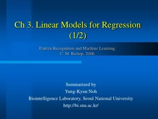
Ch 2. Probability Distributions (1/2)Pattern Recognition and Machine Learning, C. M. Bishop, 2006. Summarized by Joo-kyung Kim Biointelligence Laboratory, Seoul National University http://bi.snu.ac.kr/
Contents • 2.1. Binary Variables • 2.1.1. The beta distribution • 2.2. Multinomial Variables • 2.2.1. The Dirichlet distribution • 2.3. The Gaussian Distribution • 2.3.1. Conditional Gaussian distributions • 2.3.2. Marginal Gaussian distributions • 2.3.3. Bayes` theorem for Gaussian variables • 2.3.4. Maximum likelihood for the Gaussian • 2.3.5. Sequential estimation (C) 2007, SNU Biointelligence Lab, http://bi.snu.ac.kr/
Density Estimation • Modeling the probability distribution p(x) of a random variable x, given a finite set x1,…,xn of observations. • We will assume that the data points are i.i.d. • Fundamentally ill-posed • There are infinitely many probability distributions that could have given rise to the observed finite data set. • The issue of choosing an appropriate distribution relates to the problem of model selection. • Begins by considering parametric distributions. • binomial, multinomial, and Gaussian • Governed by a small number of adaptive parameters. • Such as the mean and variance in the case of a Gaussian. (C) 2007, SNU Biointelligence Lab, http://bi.snu.ac.kr/
Frequentist and Bayesian Treatments for the Density Estimation • Frequentist • Choose specific values for the parameters by optimizing some criterion, such as the likelihood function. • Bayesian • Introduce prior distributions over the parameters and the use Bayes` theorem to compute the corresponding posterior distribution given the observed data. (C) 2007, SNU Biointelligence Lab, http://bi.snu.ac.kr/
Bernoulli Distribution • Considering single binary r.v. x∈{0,1}. • Frequentist treatment • Likelihood function • Suppose we have a data set D={x1,…,xN} of observed values of x. • Maximum likelihood estimator • If we flip a coin 3 times and happen to observe 3 heads the ML estimator is 1. • An extreme example of the overfitting associated with ML. (C) 2007, SNU Biointelligence Lab, http://bi.snu.ac.kr/
Binomial Distribution The distribution of the number m of observations of x=1 given that the data set has size N. Histogram plot of the binomial distribution (N=10, μ=0.25) Beta Distribution Binomial & Beta Distribution (C) 2007, SNU Biointelligence Lab, http://bi.snu.ac.kr/
Bernoulli & Binomial Distribution - Bayesian Treatment (1/3) • We need to introduce a prior distribution. • Conjugacy • Posterior distribution have the same functional form as the prior. • We will use beta distribution as the prior. • The posterior distribution of μ is now obtained by multiplying the beta prior by the binomial likelihood function and normalizing. • Has the same functional dependence on μ as the prior distribution reflecting the conjugacy properties. (C) 2007, SNU Biointelligence Lab, http://bi.snu.ac.kr/
Bernoulli & Binomial Distribution - Bayesian Treatment (2/3) • Because of the beta distribution property, it is simple to normalize. • Simply another beta distribution • Observing a data set of m observations of x=1 and has been to increase the value of a by m. • This allows us to provide a simple interpretation of the hyperparameters a and b in the prior as an effective number of observations if x=1 and x=0. (C) 2007, SNU Biointelligence Lab, http://bi.snu.ac.kr/
Bernoulli & Binomial Distribution - Bayesian Treatment (3/3) • The posterior distribution can act as the prior if we subsequently observe additional data. • Prediction of the outcome of the next trial • If m,l∞, then the result reduces to the maximum likelihood result. • The Bayesian and maximum likelihood results (frequentist view) will agree in the limit of an infinitely large data set. • For a finite data set, the posterior mean for μ always lies between the prior mean and the maximum likelihood estimate for μ corresponding to the relative frequencies of events given by μML. • As the number of observations increases, the posterior distribution becomes more sharply peaked (variance is reduced). • Illustration of one step of sequential Bayesian inference (C) 2007, SNU Biointelligence Lab, http://bi.snu.ac.kr/
We will use 1-of-K scheme The variable is represented by a K-dimensional vector x in which one of the elements xk equals 1, and all remaining elements equal 0. Ex) x=(0,0,1,0,0,0)T Considering a data set D of N independent observations. Maximizing the log-likelihood using a Lagrange multiplier Multinomial distribution The joint distribution of the quantities m1,…,mK, conditioned on the parameters μ and on the total number N of observations. Multinomial Variables (C) 2007, SNU Biointelligence Lab, http://bi.snu.ac.kr/
Dirichlet distribution The relation of multinomial and Dirichlet distributions is the same as that of binomial and beta distributions. The Dirichlet distribution over three variables. Confined to a simplex because of the constraints. Two horizontal axes are simplex, the vertical axis corresponds to the density. (ak=0.1, 1, 10, respectively) Dirichlet distribution (C) 2007, SNU Biointelligence Lab, http://bi.snu.ac.kr/
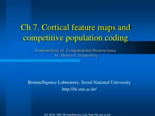
The Gaussian Distribution • In the case of a single variable • For a D-dimensional vector x • The distribution maximizes the entropy • The central limit theorem • The sum of a set of random variables has a distribution that becomes increasingly Gaussian as the number of terms in the sum increases. (C) 2007, SNU Biointelligence Lab, http://bi.snu.ac.kr/
The Geometrical Form of the Gaussian Distribution (1/3) • Functional dependence of the Gaussian on x • Δ is called the Mahalanobis distance • Is the Euclidean distance when ∑ is I. • ∑ can be taken to be symmetric. • Because any antisymmetric component would disappear from the exponent. • The eigenvector equation • Choose the eigenvectors to form an orthonormal set. (C) 2007, SNU Biointelligence Lab, http://bi.snu.ac.kr/
The Geometrical Form of the Gaussian Distribution (2/3) • The covariance matrix can be expressed as an expansion in terms of its eigenvectors • The functional dependence becomes • We can interpret {yi} as a new coordinate system defined by the orthonormal vectors ui that are shifted and rotated. (C) 2007, SNU Biointelligence Lab, http://bi.snu.ac.kr/
The Geometrical Form of the Gaussian Distribution (3/3) • y=U(x-μ) • U is a matrix whose rows are given by uiT. • Orthogonal matrix. • To be well defined, it should be positive definite. • The determinant |∑| of the covariance matrix can be written as the product of its eigenvalues. • The Gaussian distribution takes the form which is the product of D independent univariate Gaussian distributions. (C) 2007, SNU Biointelligence Lab, http://bi.snu.ac.kr/
Covariance Matrix Form for the Gaussian Distribution • For large D, the total number of parameters grows quadratically with D. • One way to reduce computation cost is to restrict the form of the covariance matrix. • (a) general form • (b) diagonal • (c) isotropic (proportional to the identity matrix) (C) 2007, SNU Biointelligence Lab, http://bi.snu.ac.kr/
Conditional & Marginal Gaussian Distributions (1/2) • If two sets of variables are jointly Gaussian, then the conditional distribution of one set conditioned on the other is again Gaussian. • The mean of the conditional distribution p(xa|xb) is a linear function of xb and covariance is independent of xa. • An example of a Linear Gaussian model. • If a joint distribution p(xa, xb) is Gaussian, then the marginal distribution is also Gaussian. • Prove using that (C) 2007, SNU Biointelligence Lab, http://bi.snu.ac.kr/
The contours of a Gaussian distribution p(xa,xb) over two variables. The marginal distribution p(xa) and the conditional distribution p(xa|xb) Conditional & Marginal Gaussian Distributions (2/2) (C) 2007, SNU Biointelligence Lab, http://bi.snu.ac.kr/
ML w.r.t. μ. ML w.r.t. ∑. Imposing the symmetry and positive definiteness constraints Evaluating the expectations of the ML solutions under the true distribution. The ML estimate for the covariance has an expectation that is less than the true value. Using following estimator, that can be corrected. Maximum likelihood for the Gaussian (C) 2007, SNU Biointelligence Lab, http://bi.snu.ac.kr/
Allow data points to be processed one at a time and then discarded. Robbins-Monro algorithm More general formulation of sequential learning Consider a pair of random variables θ and z governed by a joint distribution p(z,θ). Regression function Our goal is to find the root θ* at which f(θ*)=0. We observe z one at a time and wish to find a corresponding sequential estimation scheme for θ*. Sequential Estimation (1/2) (C) 2007, SNU Biointelligence Lab, http://bi.snu.ac.kr/
In the case of a Gaussian distribution. (Θ corresponds to μ) The Robbins-Monro procedure defines a sequence of successive estimate of the root θ*. A general maximum likelihood problem Finding the maximum likelihood solution corresponds to finding the root of a regression function. Sequential Estimation (2/2) (C) 2007, SNU Biointelligence Lab, http://bi.snu.ac.kr/