Download
1 / 56
560 likes | 680 Views
This guide provides an overview of essential statistical topics covered in the CBASE exam, crucial for success in understanding data analysis. Key areas include statistical reasoning, measures of center (mean, median, mode), measures of spread (range, standard deviation), and probability concepts like independence and mutually exclusive events. Learn about data collection methods, sample selection techniques, and the importance of representative samples. A strong foundation in these topics will help you interpret data effectively and apply statistical logic in various scenarios.

E N D
Statistics topics for CBASE Exam Dr. Glen A. Just
Major Topics • Overview • Statistical Reasoning, Misleading Data • Graphs and Visual Displays • Trends, Predictions, Extrapolation • Measures of Center (mean, median, mode) • Measures of Spread (range, standard deviation) • Probability (independence, mutually exclusive)
Overview - Basic Terms • Statistics: • A systematic method of gathering, organizing, analyzing, and interpreting data. • Collection about a particular topic or event (football, baseball, etc.) • Two Primary Sources: • Population (all possible people, experiments, observations, etc.) • Sample (subset of population) • Two Primary Types of Investigations: • Qualitative study (explorative) • Quantitative study (attempts to prove hypotheses)
Statistical Reasoning – Quantitative Studies • Statistical reasoning may be defined as the way people reason with statistical ideas and make sense of statistical information. • This involves making interpretations based on sets of data, graphical representations, and statistical summaries. • Much of statistical reasoning combines ideas about data and chance, which leads to making inferences and interpreting statistical results. • Underlying this reasoning is a conceptual understanding of important ideas, such as distribution, center, spread, association, uncertainty, randomness, and sampling.
Statistical Reasoning – Quantitative Studies • Statistical reasoning can be viewed as a three-step process: • Comprehension (seeing a particular problem as similar to a class of problems), • Planning and execution (applying appropriate methods to solve the problem), and • Evaluation and interpretation (interpreting the outcome as it relates to the original problem). • The CBASE exam focuses primarily on • statistical logic, • data representation, and • computation.
Statistical Reasoning – Sample Selection • For statistical conclusions to be valid: • A sample must be selected randomly (each element had same chance) • A sample must be representative of the population • Conclusions must be reasonable for the data gathered • Random selection methods: • Simple random selection (from a hat) • Systematic random selection (random starting point) • Stratified random selection (equal proportions)
Statistical Reasoning – Sample Selection • We want to estimate the total income of adults living in a given street. We visit each household in that street, identify all adults living there, and randomly select one adult from each household. We then interview the selected person and find their income.
Statistical Reasoning – Sample Selection • We want to estimate the total income of adults living in a given street. We visit each household in that street, identify all adults living there, and randomly select one adult from each household. We then interview the selected person and find their income. • Problem 1: People living on their own are certain to be selected, so we simply add their income to our estimate of the total. But a person living in a household of two adults has only a one-in-two chance of selection.
Statistical Reasoning – Sample Selection • We want to estimate the total income of adults living in a given street. We visit each household in that street, identify all adults living there, and randomly select one adult from each household. We then interview the selected person and find their income. • Problem 1: People living on their own are certain to be selected, so we simply add their income to our estimate of the total. But a person living in a household of two adults has only a one-in-two chance of selection. • Fix 1: To correct this, when we come to such a household, we would count the selected person's income twice towards the total. (The person who is selected from that household can be loosely viewed as also representing the person who isn't selected.)
Statistical Reasoning – Sample Selection • We want to estimate the total income of adults living in a given street. We visit each household in that street, identify all adults living there, and randomly select one adult from each household. We then interview the selected person and find their income. • Problem 1: People living on their own are certain to be selected, so we simply add their income to our estimate of the total. But a person living in a household of two adults has only a one-in-two chance of selection. • Fix 1: To correct this, when we come to such a household, we would count the selected person's income twice towards the total. (The person who is selected from that household can be loosely viewed as also representing the person who isn't selected.) • Problem 2: Not everybody has the same probability of selection; so it would not be considered a “random” selection.
Statistical Reasoning – Sample Selection • We want to estimate the total income of adults living in a given street. We visit each household in that street, identify all adults living there, and randomly select one adult from each household. We then interview the selected person and find their income. • Problem 1: People living on their own are certain to be selected, so we simply add their income to our estimate of the total. But a person living in a household of two adults has only a one-in-two chance of selection. • Fix 1: To correct this, when we come to such a household, we would count the selected person's income twice towards the total. (The person who is selected from that household can be loosely viewed as also representing the person who isn't selected.) • Problem 2: Not everybody has the same probability of selection; so it would not be considered a “random” selection. • Fix 2: Identify the wager earners in each house living along the street. Suppose that there are k wage earners. Assign each wage earner a unique number from 1 to k. Place the numbers in a “hat” and draw out 15 numbers (with replacement). “SRS”
Statistical Reasoning – Sample Selection • In 1936, the early days of opinion polling, the American Literary Digest magazine collected over two million postal surveys and predicted that the Republican candidate in the U.S. presidential election, Alf Landon, would beat the incumbent president, Franklin Roosevelt by a large margin. However, the exact opposite result occurred. What happened?
Statistical Reasoning – Sample Selection • In 1936, the early days of opinion polling, the American Literary Digest magazine collected over two million postal surveys and predicted that the Republican candidate in the U.S. presidential election, Alf Landon, would beat the incumbent president, Franklin Roosevelt by a large margin. However, the exact opposite result occurred. What happened? • Was the sample large enough (replication)?
Statistical Reasoning – Sample Selection • In 1936, the early days of opinion polling, the American Literary Digest magazine collected over two million postal surveys and predicted that the Republican candidate in the U.S. presidential election, Alf Landon, would beat the incumbent president, Franklin Roosevelt by a large margin. However, the exact opposite result occurred. What happened? • Was the sample large enough (replication)? Yes. Over two million surveys were used.
Statistical Reasoning – Sample Selection • In 1936, the early days of opinion polling, the American Literary Digest magazine collected over two million postal surveys and predicted that the Republican candidate in the U.S. presidential election, Alf Landon, would beat the incumbent president, Franklin Roosevelt by a large margin. However, the exact opposite result occurred. What happened? • Was the sample representative of the population?
Statistical Reasoning – Sample Selection • In 1936, the early days of opinion polling, the American Literary Digest magazine collected over two million postal surveys and predicted that the Republican candidate in the U.S. presidential election, Alf Landon, would beat the incumbent president, Franklin Roosevelt by a large margin. However, the exact opposite result occurred. What happened? • Was the sample representative of the population? No. There is no mention that the sample was selected randomly. The Literary Digest survey represented a sample collected from readers of the magazine, supplemented by records of registered automobile owners and telephone users. This sample included an over-representation of individuals who were rich, who, as a group, were more likely to vote for the Republican candidate.
Sample Selection – Your Turn • Sally Statistics, wants to survey the AU student body on their stand on government programs to help the poor. She decides to sit at a table in the cafeteria and asks entering students if the amount spent by the government on welfare is a. too little, b. too much, or c. about right. After she gathers 12 responses, she reports her finding to her ethics class. • Is this a good study to gauge AU perceptions?
Sample Selection – Your Turn • Sally Statistics, wants to survey the AU student body on their stand on government programs to help the poor. She decides to sit at a table in the cafeteria and asks entering students if the amount spent by the government on welfare is a. too little, b. too much, or c. about right. After she gathers 12 responses, she reports her finding to her ethics class. • Problems: • Only cafeteria users would be involved • Sample size is small • “Welfare” can be view negatively (“Assistance” is better).
Reading Graphs • The purpose of a graph is to present data in a pictorial format that is easy to understand. A graph should make sense without any additional explanation needed from the body of a report. • Graphs should not use unnecessary colors, shading, or three dimensional effects. Labeling should be adequate to make the graph informative.
Visual Representation of Data – Line Graph What is the difference between the values for February and April?
Visual Representation of Data - Table • The characteristics for a table are the same as for a graph. The purpose is to make the information more understandable for the reader. • This table could be made clearer if the definition of “Group” and “Class” were indicated. • If the table is trying to indicate a pattern, then a graph (such as a line graph) might be a better choice than this table.
Visual Representation of Data – Stem-and-Leaf • The stem-and-leaf diagram shows data values by using two groups of numbers, stems and leaves. • For this diagram, the stem of “2” with leaf of “0” represents 20. The stem of “2” with the leaf of “1” means 21. • If a leaf if repeated, that means its associated value occurred multiple times. For instance, 60 occurred twice in the data set. Leaf unit = 1 2 0 1 1 3 5 3 2 2 5 8 4 3 6 8 5 1 2 7 8 6 0 0 1 Stem units Leaf units Stem units are typically ten times the leaf units. Leaf = 1, Stem = 10.
Stem-and-Leaf – Your Turn • In the stem-and-leaf diagram to the right, what does the “3” and “1” mean? Leaf unit = 10 1 0 1 2 3 7 2 2 5 6 3 1 6 9 4 2 3 6 5 0 0 1
Stem-and-Leaf – Your Turn • In the stem-and-leaf diagram to the right, what does the “3” and “1” mean? • Since the Leaf unit is 10, the stems represent units of 100. Thus the 3 means 300 andthe 1 means 10. • “3” and “1” mean 310. Leaf unit = 10 1 0 1 2 3 7 2 2 5 6 3 1 6 9 4 2 3 6 5 0 0 1
Sometimes a display will reveal a pattern or trend Age This scatter plot shows a trend. What is it?
Sometimes a display will reveal a pattern or trend Age This scatter plot shows a trend. What is it? There is a (linear) trend for larger values for the husband’s age to be matched to larger values for the wife’s age.
Sometimes a display will reveal a pattern or trend Age Sometimes the trend is not linear. Here the trend is cyclic. In fact, there are cycles inside of cycles with this data.
Measures of Center The three most commonly used measures of center are: Mean Mode Median Mean: Sum of the data values divided by the number of data values. 1, 5, 8, 9, 12 Sum = 35 Divided by 5: 35/5 = 7 The mean is 7.
Center of the data - Mode Mode: Data value with the highest frequency (count). 1, 5, 8, 9, 12 Mode = none. No one number shows up more often than the others. 1, 5, 5, 9, 12. Mode = 5. The number 5 shows up twice. All others show up only once. 1, 5, 5, 9, 9. Modes = 5 and 9. Two numbers show up more often than the other(s). The data are bimodal.
Center of the data - Median Median: Data value in the middle of the (sorted) values. 3, 5, 8, 9, 12 Median = 8. 8 is the number that is in the middle. There are two numbers less than 8 and two numbers more than 8. 5, 9, 3, 5, 12. Median = 5. The number 3 is NOT the median because the data values were not in order (sorted). In order, the numbers are 3, 5, 5, 9,. 12. The number in the middle is 5. There are two numbers “below” 5 and two numbers above 5. 3, 5, 7, 9, 11, 12. Median = 8. When there is an even number of data values, the middle two are averaged. (7+9 ) / 2 = 16/2 = 8.
Center of the data - All For the following values, find the mean, mode, and median: 11, 14, 15, 8, 9, 15 Mean = Mode = Median =
Center of the data - All For the following values, find the mean, mode, and median: 11, 14, 15, 8, 9, 15 Mean = 12. (11+14+15+8+9+15)/6. 72/6 = 12. Mode = 15. The number 15 shows up more often (twice) than the other numbers. Median = 12.5 In order, the numbers are 8, 9, 11, 14, 15, 15. Since there is an even number of values, the middle two are averaged. (11+14)/2 = 25/2 = 12.5. The median is 12.5.
Spread of the data There are two main measures for the spread (variation) of the data values. Range: Distance from smallest to largest data values. Standard deviation: Distance the data values are away from the mean. For the following values, find the range and standard deviation: 11, 14, 15, 8, 9, 15 Range = 15 – 8 = 7. Standard deviation needs the mean: Mean = 12. (11+14+15+8+9+15)/6. 72/6 = 12. Standard deviation =
Spread of the data - standard deviation Standard deviation for the data values: 11, 14, 15, 8, 9, 15 Standard deviation needs the mean: Mean = 12. (11+14+15+8+9+15)/6. 72/6 = 12. Standard deviation =
Spread of the data - standard deviation Standard deviation for the data values: 11, 14, 15, 8, 9, 15 Standard deviation needs the mean: Mean = 12. (11+14+15+8+9+15)/6. 72/6 = 12. Standard deviation = The total of the squared values is 48. 48/5 = 9.6 The square root of 9.6 is approx. 3.1
Spread of the data – Range and Standard Deviation Find the range and standard deviation for: 6, 4, 5, 2, 3 Range = Standard deviation =
Range and Standard Deviation – Your Turn Find the range and standard deviation for: 6, 4, 5, 2, 3 Range = 6 – 2 = 4. Standard deviation =
Spread of the data – Range and Standard Deviation Find the range and standard deviation for: 6, 4, 5, 2, 3 Range = 6 – 2 = 4. Standard deviation needs the mean: Mean = 4. (6+4+5+2+3)/5. 20/5 = 4. Standard deviation =
Spread of the data – Range and Standard Deviation Find the range and standard deviation for: 6, 4, 5, 2, 3 Standard deviation needs the mean: Mean = 4. Standard deviation = The total of the squared values is 10. 10/4 = 2.5 The square root of 2.5 is approx. 1.58.
Probability – Events and Likelihood Probability is the likelihood (chance) of something happening. If 3 red marbles and 2 blue marbles are placed in a bag and you draw out one marble (without looking), the probability that the marble is red is 3/5 or 60%. Likewise, the probability of withdrawing a blue marble is 2/5 or 40%. The probability of having a male child is 50%. A couple has two children, both of whom are male. What is the probability that the couple’s third child will be male? 0.125 0.50 1.00 1.25
Probability – Events and Likelihood Probability is the likelihood (chance) of something happening. If 3 red marbles and 2 blue marbles are placed in a bag and you draw out one marble (without looking), the probability that the marble is red is 3/5 or 60%. Likewise, the probability of withdrawing a blue marble is 2/5 or 40%. The probability of having a male child is 50%. A couple has two children, both of whom are male. What is the probability that the couple’s third child will be male? 0.125 0.50 (Correct answer. The probability is the same for each child.) 1.00 1.25 (This is not a valid probability 0 probability 1. )
Probability – Multiple Events (AND) Two or more events can be combined. The probability of the combined events can be computed using a few formulas. “AND” Probability of A and B. (Independent events) Let “A” mean flipping a coin and getting a “head”. Let “B” mean rolling a die and getting a “3”. Since A and B have no connection (independent), P(A and B) = P(A)P(B) = (1/2)(1/6) = 1/12 = 0.8333…
Probability – Multiple Events (AND) “AND” Probability of A and B. (Dependent events) Suppose we place 3 red marbles and 2 blue marbles in a bag. Let “A” mean drawing out a red marble (without looking). Let “B” mean drawing out a blue marble (without looking and without replacing the first “red” marble). Since A and B have a connection they are dependent, P(A and B) = P(A)P(B, given A) = (3/5)(2/4) = 3/10 = 0.3 Note: If the first marble was replaced, then the events would be independent, P(A and B) = P(A)P(B, given A) = (3/5)(2/5) = 6/25 = 0.24