Computational Genome Annotation
Computational Genome Annotation. Chapter 3 Ying Xu. Introduction. DNA sequence of a genome encodes the entire functionality , Millions (microbes) to Billions (human), What information is encoded in a cont., A’s, C’s, G’s and T’s string? Where it is located ?

Computational Genome Annotation
E N D
Presentation Transcript
Computational Genome Annotation Chapter 3 Ying Xu
Introduction • DNA sequence of a genome encodes the entire functionality, • Millions (microbes) to Billions (human), • What information is encoded in a cont., A’s, C’s, G’s and T’s string? • Where it is located ? • What information is identifiable directly ? • How should the identified directly information be presented ? • Two approaches, 1. Ab initio approach, 2. Comparative approach.
Ab initio -> predicts functional elements by statistical features and used to identify novel functional elements, • Comparative approach -> sequence similarity to previously known one.
3.2 Prediction of Protein-Coding genes • Single largest set of functional elements in a genome consists of genes, • 75-90%of microbial genome contains gene-coding regions, • Sequence fragment between two stop codonsof the same reading frame is called an open reading frame (ORF),
3.2.1 Evaluation of coding potential • Abinitio prediction - based on di-codons, or six-mers, • Eg., di-codonGACTGC, largely occur in noncodingregions than in coding regions in Shewanellaoneidensis, • 4,096 different di-codonsin a genome ( 46 = 4,096),
For each di-codon X • Total numbers of occurrences of X in coding and noncodingregions. • Relative frequency (RF)of X in coding regions = number of occurrences of X / total number in coding regions • Est. RF of X in non-coding regions in a similar fashion.
Preference model • Log(FC(X)/FN(X)), • FC(X) X’s relative frequency in a coding region • FN(X) X’s relative frequency in a noncoding region, • If X have the same RF - preference value is zero. • Positive value - X has a higher RF in coding than in a non-coding region; • otherwise, it will be negative
Overall preference value = sum of all preference values of the di-codons. • Positive preference value -> coding region • Negative preference value -> noncoding region. • GRAIL AND SORFIND, • HIDDEN MARKOV MODELS,
Markov Chain Model • Consecutive 6-mers or di-codons are independent, • Modeling dependence relationships among consecutive di-codons,
Baysian formula • P(S = s1, s2, . . . , sk|coding) and P(S = s1, s2, . . . , sk|noncoding) probability of DNA segment S = s1, s2, . . . , sk. • P(coding|S) = P(S|coding)/(P(S|coding) + P(S|noncoding)P(noncoding)/P(coding)) fifth-order model
3.2.2 Identification of translation start • Similar sequence patterns around the ATG, • Predict new translation starts based on previously known, • Weight matrix, • Flanking DNA sequence
3.2.3 Ab initio Gene Prediction through Information Fusion • Identify all ORFs in six reading frames, • Measure the coding potential, • High translation-start score and the whole region has high coding potential • Strong coding potential on right and low coding potential on left.
Gene Length Distribution • Length distribution of all known genes is not uniform. • Exponential distribution or a gamma distribution. • Asymmetric and heavy tail on the right side.
G+C Composition • Different G+C compositions have different di-codonfrequencies, • One set of di-codon RF lead to incorrect predictions. • Different di-codon frequency tables . • Normalization factor.
Regions of Repeats • Not overlap with any genes, • Reliable prediction software programs, • These regions are maskedout before running a gene-finding program.
Neural Networking • A non-gene is a region in an ORF that does not overlap any coding regions • set A contains only genes and set B contains only non-genes, • Examine the common features of sets A & B
set A consists of a list of vectors (C1, C2, T, G, L, 1) for each gene • set B consists of a list of (C1, C2, T, G, L, 0) for each nongene. • 0 and 1 - one set consists of all genes and the other set all nongenes.
Back-propagation • One or two hidden layers should suffice. • Nodes are connected with edges. • Adjusting the edge weights. • GRAIL - main prediction framework.
Web Servers for Genome Annotation neural network Output node Hidden layer InputNodes
3.2.4 Gene Identification through comparative analysis • High sequence similarity • BLAST • First Comparative approach to find a subset of genes • Ab initio method to find the rest of the genes in the genome. • EST-based Gene Predictions
Identifying Conserved Regions across Multiple Genomes • Conserved (long) regions across multiple genomes,
PatternHunter • Non-contiguou sequence matches. • Very less time and memory requirement, than BLAST. • DIALIGN - predicts genes through genome-scale sequence comparison Genome A Genes Genome B
3.2.5 Interpretation of Gene Prediction • GRAIL : marginal, intermediate, or strong descriptors, • All predictions divide into bins based on the prediction scores. • Genes with scores between 0 and 0.1 are put into the first bin, • All genes with scores between 0.1 and 0.2 in the second bin, etc.
Cont., • Different reliability thresholds applied for different purposes. • Gene validation, consider a high reliability threshold, • General screening - Low reliability threshold.
Pseudogenes • Frameshifts due to deletions/insertions, • Hard for a regular gene prediction program. • Specialized coding-region detection program, • Mycobacterium leprae has 1,100 predicted pseudogenes
3.3 PREDICTION OF RNA-CODING GENES • tRNA (transfer RNA), rRNA (ribosomal RNA), sRNA (small RNA), srpRNA (signal recognition particle RNA), etc. • Catalyst and information storage molecules. • tRNAs adapter molecules that decode the genetic code. • rRNA catalyze the synthesis of proteins.
Cont., • (1) RNA signals are a combination of sequence and structure motifs. • for example, tRNA genes designed to recognize particular types of RNA genes.
Cont., ` • (2) Secondary structures in its folded tertiary structure, • Stems, provide signals for RNA gene recognition, • tRNAscan-SE, • Accuracy greater than 99%, • False positive rate at one false prediction per 15 gigabases.
Secondary structure Loops Stem
3.4 IDENTIFICATION OF PROMOTERS • Coding regions and Regulatory regions, • mRNA transcription, • Transcription process is initiated by RNA polymerase.
3.4.1 Promoter Prediction through Feature Recognition • Hidden Markov model (HMM) - statistical tool, • Promoter sequences have higher probabilities than that of nonpromoter sequences. • Conserved sequence fragments and their spacing relationships.
CONSENSUS • Conserved k-mers • Determine if the current sequence contains any k-mers that are similar to any k-mers of the previous sequences • Consensus matrix.
MEME • Maximum likelihood of the conserved k-mers - EM algorithm • Signal Scan and NNPP • Promoter-gene structure or the more general structure of promoter-gene-gene- . . . -gene
3.5 OPERON IDENTIFICATION • A basic organizational unit of genes, • transcriptional regulation. • Genes in an operon are tandem and controlled by a regulatory binding motifs
Computational identification of an operon (1) Predicte promoter region and a terminator, (2) Set of genes arranged in tandem on the same strand, (3) Functional information of the genes involved. • Identify transcriptional regulatory networks
Terminator Identification • rho-dependent and rho-independent, Three nucleic acid binding sites : • A double-stranded DNA binding site, • An RNA–DNA hybrid binding site, • A single-stranded RNA binding site.
TransTerm • Finds rho-independent transcription terminators ( Bacterial genomes ). • Catalyze successive reactions in metabolic pathways, • http://genomics4.bu.edu/operons/,
Cont., • lacoperon. • trpoperon biosynthesis of tryptophan • mhpoperon phenylpropionate catabolic pathway • Using these known operons, 1) Intergenetic distance within an operon vs. between operons, (2) Distribution of the number of genes
3.6 FUNCTIONAL CATEGORIES OF GENES • EC classes for enzymes, • An ad hoc way, • If “Metabolism” or “pathway”, of gene is known, its functional category will be labeled.
Functional assignments of genes in the “cell motility” pathway
3.7 CHARACTERIZATION OF OTHER FEATURES IN A GENOME • G + C Composition: Correlates with density of genes, • In a genome, higher G + C compositions imply higher gene densities.
CpG Islands • DNA with a higher frequency of CpGdinucleotides. • Transcriptional starts of genes. • Commonly used threshold is 0.6. • Human genome threshold is 0.8,
Genomic Repeats • Prokaryotic and eukaryotic genomes. • Transposons- mobile elements to move around a genome. • Genome annotation process. • Gene density: Number of genes per fixed length of genomic sequence.
Cont., • (a) Tandem Repeat Identification: Exact and approximate string matching. • (b) RepeatMasker: Matching all the repeat sequences in its database against the DNA sequence. • (c) RepeatFinder: Either exact or approximate match, using a clustering technique.
3.8 GENOME-SCALE GENE MAPPING • Genes Unique to a Genome: 20 to 30% of genes in a genome are unique. • Genome Rearrangement: One gene’s location differ from their corresponding genes • Quantitative studies of genome.
Cont., • Reversal Distance: Defined from (a, b) to (b,a), where b1, b2, . . . , bn is a permutation of a1, a2, . . . , an. • Transposition Distance: Block of genes from one position to another.