Transportation Problems
Transportation Problems. MHA 6350. Medical Supply Transportation Problem. A Medical Supply company produces catheters in packs at three productions facilities. The company ships the packs from the production facilities to four warehouses.

Transportation Problems
E N D
Presentation Transcript
Transportation Problems MHA 6350
Medical Supply Transportation Problem • A Medical Supply company produces catheters in packs at three productions facilities. • The company ships the packs from the production facilities to four warehouses. • The packs are distributed directly to hospitals from the warehouses. • The table on the next slide shows the costs per pack to ship to the four warehouses.
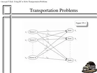
Source: Adapted from Lapin, 1994 Medical Supply TO WAREHOUSE FROM PLANT Seattle New York Phoenix Miami Juarez $19 $ 7 $ 3 $21 Seoul 15 21 18 6 Tel Aviv 11 14 15 22 Capacity Juarez 100 Seoul 300 Tel Aviv 200 Demand Seattle 150 New York 100 Phoenix 200 Miami 150
Source: Adapted from Lapin, 1994 From Plant TO WAREHOUSE Plant Capacity S N P M J Xjs Xjn Xjp Xjm 100 S Xss Xsn Xsp Xsm 300 T Xts Xtn Xtp Xtm 200 Warehouse Demand 150 100 200 150 600 Number of constraints = number of rows + number of columns Total plant capacity must equal total warehouse demand. Although this may seem unrealistic in real world application, it is possible to construct any transportation problem using this model.
J 100 S 300 T 200 Source: Adapted from Lapin, 1994 Northwest Corner Method S N P M Capacity To From 19 7 3 21 15 21 18 6 11 14 15 22 Demand 150 100 200 150 600 Begin with a blank shipment schedule. Note the shipping costs in the upper right hand corner of each cell.
J 100 S 300 T 200 Source: Adapted from Lapin, 1994 Northwest Corner Method S N P M Capacity To From 19 7 3 21 100 15 21 18 6 11 14 15 22 Demand 150 100 200 150 600 Start in the upper left-hand corner, “northwest corner” of the schedule and place the largest amount of capacity and demand available in that cell. Seattle demands 150 and Jaurez has a capacity of 100.
J 100 S 300 T 200 Source: Adapted from Lapin, 1994 Northwest Corner Method S N P M Capacity To From 19 7 3 21 100 15 21 18 6 50 11 14 15 22 Demand 150 100 200 150 600 Since Juarez capacity is depleted move down to repeat the process for the Seoul to Seattle cell. Seoul has sufficient capacity but Seattle can only take another 50 packs of demand.
J 100 S 300 T 200 Source: Adapted from Lapin, 1994 Northwest Corner Method S N P M Capacity To From 19 7 3 21 100 15 21 18 6 50 100 150 11 14 15 22 50 150 Demand 150 100 200 150 600 Now move to the next cells to the right and assign capacity for Seoul to warehouse demand until depleted. Then move down to the Tel Aviv row and repeat the process.
J 100 S 300 T 200 Source: Adapted from Lapin, 1994 Northwest Corner Method S N P M Capacity To From 1900 750 2100 2700 750 3300 C =11,500 19 7 3 21 1900 15 21 18 6 750 2100 2700 11 14 15 22 750 3300 Demand 150 100 200 150 600 The previous slides show the process of satisfying all constraints and allows us to begin with a starting feasible solution. Multiply the quantity in each cell by the cost.
S N P M Capacity To From 19 7 3 21 100 J 100 15 21 18 6 S 300 50 100 150 T 200 11 14 15 22 50 150 Demand 150 100 200 150 600 Source: Adapted from Lapin, 1994 For non empty cells: cij = ri+ kj Assign zero as the row number for the first row. rj = 0 a ks = 19 19 = (0) + ks b
S N P M Capacity To From 19 7 3 21 100 J 100 15 21 18 6 S 300 50 100 150 T 200 11 14 15 22 50 150 Demand 150 100 200 150 600 Source: Adapted from Lapin, 1994 For non empty cells: cij = ri+ kj Assign zero as the row number for the first row. rj = 0 a c rs = -4 ks = 19 15 = rs + 19 rs = -15 + 19 = -4 b Note: Always use the newest r value to compute the next k.
S N P M Capacity To From 19 7 3 21 100 J 100 15 21 18 6 S 300 50 100 150 * T 200 11 14 15 22 50 150 Demand 150 100 200 150 600 Source: Adapted from Lapin, 1994 For non empty cells: cij = ri+ kj Assign zero as the row number for the first row. rj = 0 a c rs = -4 ks = 19 kp = 22 18 =-4 + kp 18 + 4 = kp = 22 b d Skip cell SN, mark it * for later and move on to cell SP .
S N P M Capacity To From 19 7 3 21 100 J 100 15 21 18 6 S 300 50 100 150 * T 200 11 14 15 22 50 150 Demand 150 100 200 150 600 Source: Adapted from Lapin, 1994 For non empty cells: ctp = rt+ kp Assign zero as the row number for the first row then use the newest r value to compute the next k. rj = 0 a c rs = -4 rt = -7 e ks = 19 kp = 22 15 = rt + 22 15 - 22 = rt = -7 b d
S N P M Capacity To From 19 7 3 21 100 J 100 15 21 18 6 S 300 50 100 150 * T 200 11 14 15 22 50 150 Demand 150 100 200 150 600 Source: Adapted from Lapin, 1994 For non empty cells: cij = ri+ kj Assign zero as the row number for the first row then use the newest r value to compute the next k. rj = 0 a c rs = -4 rt = -7 e ks = 19 kp = 22 km = 29 22 = -7 + km 22 + 7 = km = 29 b d f
S N P M Capacity To From 19 7 3 21 100 J 100 15 21 18 6 S 300 50 100 150 * T 200 11 14 15 22 50 150 Demand 150 100 200 150 600 Source: Adapted from Lapin, 1994 For non empty cells: cij = ri+ kj Assign zero as the row number for the first row then use the newest r value to compute the next k. rj = 0 a c rs = -4 rt = -7 e ks = 19 kn = 25 kp = 22 km = 29 21= -4 + kn 21 + 4 = kn = 25 b g d f
S N P M Capacity To From 19 7 3 21 100 J 100 15 21 18 6 S 300 50 100 150 T 200 11 14 15 22 50 150 Demand 150 100 200 150 600 Source: Adapted from Lapin, 1994 Next calculate empty cells using: cij - ri - kj Improvement Difference >> JN = 7 – 0 – 25 = -18 rj = 0 a -18 c rs = -4 rt = -7 e ks = 19 kn = 25 kp = 22 km = 29 b g d f
S N P M Capacity To From 19 7 3 21 100 J 100 15 21 18 6 S 300 50 100 150 T 200 11 14 15 22 50 150 Demand 150 100 200 150 600 Source: Adapted from Lapin, 1994 Next calculate empty cells using: cij - ri - kj Improvement Difference >> JP = 3 – 0 – 22 = -19 rj = 0 a -18 -19 c rs = -4 rt = -7 e ks = 19 kn = 25 kp = 22 km = 29 b g d f
S N P M Capacity To From 19 7 3 21 100 J 100 15 21 18 6 S 300 50 100 150 T 200 11 14 15 22 50 150 Demand 150 100 200 150 600 Source: Adapted from Lapin, 1994 Next calculate empty cells using: cij - ri - kj Improvement Difference >> JM = 21 – 0 – 29 = -8 rj = 0 a -18 -19 -8 c rs = -4 rt = -7 e ks = 19 kn = 25 kp = 22 km = 29 b g d f
S N P M Capacity To From 19 7 3 21 100 J 100 15 21 18 6 S 300 50 100 150 T 200 11 14 15 22 50 150 Demand 150 100 200 150 600 Source: Adapted from Lapin, 1994 Next calculate empty cells using: cij - ri - kj Improvement Difference >> SM = 6 – (-4) – 29 = -19 rj = 0 a -18 -19 -8 c rs = -4 -19 rt = -7 e ks = 19 kn = 25 kp = 22 km = 29 b g d f
S N P M Capacity To From 19 7 3 21 100 J 100 15 21 18 6 S 300 50 100 150 T 200 11 14 15 22 50 150 Demand 150 100 200 150 600 Source: Adapted from Lapin, 1994 Next calculate empty cells using: cij - ri - kj Improvement Difference >> TS = 11 – (-7) – 19 = -1 rj = 0 a -18 -19 -8 c rs = -4 -19 rt = -7 e -1 ks = 19 kn = 25 kp = 22 km = 29 b g d f
S N P M Capacity To From 19 7 3 21 100 J 100 15 21 18 6 S 300 50 100 150 T 200 11 14 15 22 50 150 Demand 150 100 200 150 600 Source: Adapted from Lapin, 1994 Next calculate empty cells using: cij - ri - kj Improvement Difference >> TN = 14 – (-7) – 25 = -4 rj = 0 a -18 -19 -8 c rs = -4 -19 rt = -7 e -1 -4 ks = 19 kn = 25 kp = 22 km = 29 b g d f
S N P M Capacity To From 19 7 3 21 100 J 100 15 21 18 6 S 300 50 100 150 T 200 11 14 15 22 50 150 Demand 150 100 200 150 600 Source: Adapted from Lapin, 1994 Next calculate empty cells using: cij - ri - kj Improvement Difference >> rj = 0 a -18 -19 -8 c rs = -4 -19 rt = -7 e -1 -4 ks = 19 kn = 25 kp = 22 km = 29 b g d f
J 100 S 300 T 200 Source: Adapted from Lapin, 1994 Next calculate the entering cell by finding the empty cell with the greatest absolute negative improvement difference. Cells JP and SM are tied for the greatest improvement at $19 per pack. Break the tie and arbitrarily choose JP. JP becomes the entering cell. Place a + sign in cell JP S N P M Capacity To From 19 7 3 21 100 rj = 0 100 (-) (+) -18 -19 -8 15 21 18 6 50 100 150 (+) (-) rs = -4 -19 11 14 15 22 50 150 rt = -7 -1 -4 Demand 150 100 200 150 600 ks = 19 kn = 25 kp = 22 km = 29 Note: Except for the entering cell all changes must involve nonempty cells.
J 100 S 300 T 200 Source: Adapted from Lapin, 1994 Continue around the closed loop until all tradeoffs are completed. Previous cost was $11,500 and the new is: S N P M Capacity To 300 2250 2100 900 750 3300 C = $9,600 From 19 7 3 21 100 rj = 0 (-) (+) -18 -19 -8 15 21 18 6 50 150 50 100 (+) (-) rs = -4 -19 11 14 15 22 50 150 rt = -7 -1 -4 Demand 150 100 200 150 600 ks = 19 kn = 25 kp = 22 km = 29 Note: Except for the entering cell all changes must involve nonempty cells.
J 100 S 300 T 200 Source: Adapted from Lapin, 1994 Begin another iteration choosing the empty cell with the greatest absolute negative improvement difference. >>>>>SM S N P M Capacity To From 19 7 3 21 100 rj = 0 19 1 11 15 21 18 6 50 150 50 100 (-) (+) rs = 15 -19 11 14 15 22 150 50 (+) (-) rt = 12 -1 -4 Demand 150 100 200 150 600 ks = 0 kn = 6 kp = 3 km = 10 Note: The r and k values and the improvement difference values have changed.
J 100 S 300 T 200 Source: Adapted from Lapin, 1994 Begin another iteration choosing the empty cell with the greatest absolute negative improvement difference. SM Previous cost was $9,600, now the new is: S N P M Capacity To 300 2250 2100 300 1500 2200 C = $8,650 From 19 7 3 21 100 rj = 0 19 1 11 15 21 18 6 50 50 150 50 100 (-) (+) rs = 15 -19 11 14 15 22 100 150 100 50 (+) (-) rt = 12 -1 -4 Demand 150 100 200 150 600 ks = 0 kn = 6 kp = 3 km = 10 Note: The r and k values and the improvement difference values have changed.
J 100 S 300 T 200 Source: Adapted from Lapin, 1994 Begin another iteration choosing the empty cell with the greatest absolute negative improvement difference. SM Previous cost was $8,650, now the new is: S N P M Capacity To 300 2250 900 1400 1500 C = $6,350 From 19 7 3 21 100 rj = 0 0 -18 11 15 21 18 6 50 100 150 150 50 (-) (+) rs = -4 -19 11 14 15 22 0 100 100 100 (+) (-) rt = 12 -20 -23 Demand 150 100 200 150 600 ks = 19 kn = 25 kn = 2 kp = 3 km = 10 Note: The r and k values and the improvement difference values have changed.
J 100 S 300 T 200 Source: Adapted from Lapin, 1994 Begin another iteration choosing the empty cell with the greatest absolute negative improvement difference. SM $6,350 S N P M Capacity To 300 2250 900 1400 1500 C = $6,350 From 19 7 3 21 100 rj = 0 20 5 31 15 21 18 6 150 150 (-) (+) rs = 16 3 -1 11 14 15 22 0 100 100 (+) (-) rt = 12 20 Demand 150 100 200 150 600 ks = -1 kn = 2 kp = 3 km = 10 Note: The r and k values and the improvement difference values have changed.
J 100 S 300 T 200 Source: Adapted from Lapin, 1994 Optimal Solution In five iterations the shipping cost has moved from $11,500 to $6,250. There are no remaining empty cells with a negative value. $6,250 S N P M Capacity To 300 750 1800 900 1100 1400 C = $6,250 From 19 7 3 21 100 rj = 0 19 4 30 15 21 18 6 50 100 150 (-) (+) rs = 15 3 11 14 15 22 100 100 (+) (-) rt = 11 1 20 Demand 150 100 200 150 600 ks = 0 kn = 3 kp = 3 km = -9 Note: The r and k values and the improvement difference values have changed.