Download
1 / 29
290 likes | 432 Views
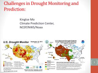
Objective Drought Monitoring and Prediction Recent efforts at Climate Prediction Ct. Kingtse Mo & Jinho Yoon Climate Prediction Center. Objectives. Develop objective drought monitoring and prediction based on drought indices Support drought monitor and outlook operation

E N D
Objective Drought Monitoring andPredictionRecent efforts at Climate Prediction Ct. Kingtse Mo & Jinho Yoon Climate Prediction Center
Objectives • Develop objective drought monitoring and prediction based on drought indices • Support drought monitor and outlook operation • Develop regional applications with users and the River Forecast Centers
Outline of presentation • Current operation Drought briefing each month (8-11 of the month, dial in is available) • If you would like to participate, email • Kingtse.mo@noaa.gov • Uncertainties of drought indices • Prediction of SPI • Future plan
Define drought based on Drought Indices • Meteorological drought: Precipitation deficit. Index: Standardized Precipitation Index • Hydrological drought: Runoff deficit Index: Standardized runoff index • Agricultural drought: Soil moisture deficit Index: SM anomaly percentile
SPI SPI3: SPI3 shows dryness over the Great Lake area Wetness over AZ, New Mexico and western Texas. For longer terms A very wet picture over the Southeast and eastern central United States D3 D2 D1
Multi model SM percentiles Feb 2010 U. Washington NCEP Univ of Washington Uncertainties in the NLDAS
Differences between two systems are larger than the spread among members of the same system • The differences are not caused by one model. They are caused by forcing. • In general, extreme values from the UW (Green) are larger than from the NCEP (red) standardized SM anomalies for area 38-42N,110-115W NCEP(red),UW(green)
Number of station P reports averaged over a year Historical period Real time Reports dropped for real time operation
Southeast & CBRFC pilot projectsEnsemble hydrologic Forecasts in support of NIDIS CPC: Kingtse Mo, Jinho Yoon EMC: Michael Ek, Youlong Xia Princeton University : Eric Wood SERFC: John Schmidt, John Feldt ,Jeff Dobur OHD: John Schaake and D. J. Seo CBRFC: Kevin Werner Funded by TRACS program
75-85W,31-35N A wet region 6 mo running mean black line drought 3 mo running mean (black line) No smoothing Red line: monthly mean, no smoothing
6 mo running mean A dry region
Hydrologic prediction Develop hydrologic forecasts out to 6 months for drought indices • P , Tmin and Tmax from the CFS forecasts=> downscaling (from 250km to 50km) and error correction=> Vic model=> SM % and runoff Based on the Princeton System developed by Eric Wood’s group • Corrected P => append P time series=> SPI indices
Linear Interpolation • Linear Interpolation : correct mean Correct the model climatology and bilinear interpolation to a high resolution grid For variable A ensemble fcst: assume normal distribution anomaly A’ rwt to model climatology A’= A-model climatology Corrected A = A’+ observed climatology
Bias correction & Downscaling (BCSD) Probability mapping based on distributions • Get probability distribution PDFs for A (coarse) and A(fine) • From A’ (coarse) get percentile based on PDF (coarse) • => assume the same percentile for the fine grid and work backward based on the PDF fine get A’ fine (anomaly) • If normally distributed , time ratio of std Ref Wood et al (U. Washington 2002,2006)
Schaake’s linear regression • Schaake’s linear regression – calibrate P ensemble forecasts based on the historical performance Do no harm Ref: Wood and Schaake (2008) Schaake et al. (2007)
Bayesian merging & bias correction • Bayesian correction – calibrate P forecast based on the historical performance and spread of members in the forecast ensemble • use all members in the ensemble Ref: Luo et al. (2007); Luo and Wood (2008)
Standardized Precipitation Index Forecasts • Append the bias corrected and downscaled P to the observed P time series • Calculate SPI from extended time series • The advantages are (1) no need of hydrologic model and (2) can use any base period. P :time series : Jan1950-oct1981 append fcsts with ICs in Oct lead 1 f1 lead 2 f2 etc Jan1950-oct 1981 (obs) Nov 1981 (fcst)
1.For the first 3 months, AC>0.6 and RMS < 0.8 2.Overall, Bayesian wins 3. Skill is higher for Nov ICs and low for May ICs Seasonal dependence of skill LI BCSD Schaake Bayesian
SPI6 T62 RMSE LI Bayesian Nov Dec Jan Feb
SPI6 T62 rmse LI Bayesian May June July Aug
Over the Southeast, SPI6 out to 3 months
SPI6 fcst (contours) /ana (colored) 32-40N Hovmoller
High resolution run (T382)and dynamic downscaling (RSM) • High resolution T382 run from April 19-23 ICs run through Nov(5 members) (Thanks Jae Schemm) • RSM (regional spectral model) downscaling from the CFS forecasts (April 28-May 3) ICs (50 km resolution) (Thanks, Henry Juang)
T62 LI 5 members vs T382 T62 15ensm LI 5 member T382 & T62 Bayesian 15 members T62 vs RSM 5 mem LI, T62 15 member LI 5 member RSM & T62 Bayesian 15 members
JJA P anom over the Northern Plains (34-42N, 100-85W) mm/day BCSD, RSM or T382, Obs mm/day
Future plan &our needs • Develop real time prediction of SPI’s based on the CFSRR hindcasts • The bias corrected P and T will drive VIC model to produce hydrologic forecasts of soil moisture and runoff • Develop regional applications with the RFCs What do we need? • Better station reporting of real time P • Better P analyses • Better global model prediction of P • Better model physics
Discussion questions • What current activities (monitoring and forecasts) can we build on? • Regional vs entire United States • How can we network and coordinate drought related information such as drought impact, planning and information exchange? • What gaps do we need to fill? • What issues are important to you, but have not been discussed?
Streamflow fcsts the binary event for observed monthly mean Row 2-6 represents the exceedence probability for forecasts initialized from Nov 2006 Luo and Wood