Download
1 / 19
190 likes | 250 Views
Learn about modeling heteroscedasticity by exploring variance functions at different levels and how to estimate separate variances for different groups. Understand the flexible notations and methods used to build these models.

E N D
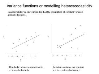
y y -3 -2 -1 0 1 2 3 x x Variance functions or modelling heteroscedasticity In earlier slides we saw our models had the assumption of constant variance – homoskedasticity… -3 -2 -1 0 1 2 3 Residuals variance constant wrt to x: homoskedasticity Residuals variance not constant wrt to x: heteroskedasticity
A simple case of heteroskedasticity In the educational data set we have been working with. Tabulating normexam by gender we see that the means and variances for boys and girls are (–0.140 and 1.051) and (0.093 and 0.940). We may want to fit a model that estimates separate variances for boys and girls. The notation we have been using so far assumes a common intercept(0) and a single set of student residuals, ei, with a common variance e2. We need to use a more flexible notation to build this model.
Working with general notation in MLwiN A model with no variables specified in general notation looks like this. A new first line is added stating that the response variable follows a Normal distribution. We now have the flexibility to specify alternative distributions for our response. We will explore these models later. The 0 coefficient now has an explanatory x0 associated with it. The values x0 takes determines the meaning of the 0 coefficient. If x0 is a vector of 1s then 0 will estimate an intercept common to all individuals, in the absence of other predictors this would be the overall mean. If x0 variable, say 1 for boys and 0 for girls, then 0 will estimate the mean for boys.
A simple variance function The new notation allows us to set up this simple model where x0i is a dummy variable for boy and x1i is a dummy variable for girl. This model estimates separate means and variances for the two groups. This is an example of a variance function because the variance changes as a function of explanatory variables. The function is :
Deriving the variance function We arrive at the expression (1)
Can be rewritten as So the between school variance is Variance functions at level 2 The notion of variance functions is powerful and not restricted to level 1 variances – we have met level 2 variance function already. The random slopes model fitted earlier produces the following school level predictions which show school level variability increasing with intake score. The model
Two views of the level 2 variance Given x0 = [1], we have Which shows that the level 2 variance is polynomial function of x1ij • View 1: In terms of school lines predicted intercepts and slopes varying across schools. ·View 2 : In terms of a variance function which shows how the level 2 variance changes as a function of 1 or more explanatory variables.
2 schools 2 students Elaborating the level 1 variance Maybe the student level departures around their schools summary lines are not constant. Note at level 2 we have 2 interpretations of level 2 random variation, random coefficients (varying slopes and intercepts across level 2 units) and variance functions. In each level 1 unit, by definition, we only have one point, therefore the first interpretation does not exist because you cannot have a slope given a single data point.
The resulting graph shows decreasing level 1 variance wrt standlrt extenuates the importance of school level factors driving variation in the outcome score, particularly for high ability pupils So the student level variance is now: Variance functions at level 1 If we allow standlrt(x1ij) to have a random term at level 1, we get
The global mean is predicted by The jth school mean is predicted by The student level variance is Where as ordinary regression: The school level variance is estimates the global relationship and has a single catch all bucket for the variance. Modelling the mean and variance simultaneously In our model
MM Opening up new types of research question Multilevel approach allows modelling of mean and variance simultaneously. Illustrate by an analysis exploring the sources of differential parenting. Why do parents treat siblings differently? Understanding the sources of differential parenting: the role of child and family level effects. Jenny Jenkins, Jon Rasbash and Tom O’Connor Developmental Psychology 2003(1) 99-113
Is there a family effect? Recent studies in developmental psychology and behavioural genetics emphasise non-shared environment and genetic influences are much more important in explaining children’s adjustment than shared environment has led to a focus on non-shared environment.(Plomin et al, 1994; Turkheimer&Waldron, 2000)
Differential parental treatment • One key aspect of the non-shared environment that has been investigated is differential parental treatment of siblings. • Differential treatment predicts differences in sibling adjustment • What are the sources of differential treatment? • Child specific/non-shared: age, temperament, biological relatedness • Can family level shared environmental factors influence differential treatment?
“Parents have a finite amount of resources in terms of time, attention, patience and support to give their children. In families in which most of these resources are devoted to coping with economic stress, depression and/or marital conflict, parents may become less consciously or intentionally equitable and more driven by preferences or child characteristics in their childrearing efforts”. Henderson et al 1996.This is the hypothesis we wish to test. We operationalised the stress/resources hypothesis using four contextual variables: socioeconomic status, single parenthood, large family size, and marital conflict The Stress/Resources Hypothesis Do family contexts(shared environment) increase or decrease the extent to which children within the same family are treated differently?
Overall mean A multilevel analysis A model for the mean and a model for the variability around the mean. positive parenting Overall mean Family means (between family variance) Child specific parenting scores vary around family mean(between child within family variance) – the within family variance is a measure of differential parental treatment.
Modelling the mean and variance simultaneously We show a possible pattern of how the mean, within family variance and between family variance might behave as functions of HSES in the schematic diagram below. Here are 5 families of increasing HSES(in the actual data set there are 3900 families. We can fit a linear function of SES to the mean. positive parenting The family means now vary around the dashed trend line. This is now the between family variation; which is pretty constant wrt HSES HSES However, the within family variation(measure of differential parenting) decreases with HSES – this supports the SR hypothesis.
Full Combined model for mean and variance • We then allow the level 1 variance to be a function of the family level variables household socioeconomic status, large family size, and marital conflict. That is Reduction in the deviance with 7df is 78.
Conclusion for differential parenting • We have found strong support for the stress/resources hypothesis. That is although differential parenting is a child specific factor that drives differential adjustment, differential parenting itself is influenced by family as well as child specific factors. • This challenges the current tendency in developmental psychology and behavioural genetics to focus on child specific factors. • Multilevel models fitting complex level 1 variation needs to be employed to uncover these relationships.