Download

1 / 66
660 likes | 776 Views
Comparing Logit and Probit Coefficients between Models and Across Groups. Richard Williams Notre Dame Sociology rwilliam@ND.Edu September 2011. Introduction.

E N D
Comparing Logit and Probit Coefficients between Models and Across Groups Richard Williams Notre Dame Sociology rwilliam@ND.Edu September 2011
Introduction • We are used to estimating models where an observed, continuous independent variable, Y, is regressed on one or more independent variables, i.e. • Since the residuals are uncorrelated with the Xs, it follows that
As you add explanatory variables to a model, the variance of the observed variable Y stays the same in OLS regression. As the explained variance goes up, the residual variance goes down by a corresponding amount.
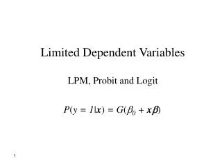
But suppose the observed Y is not continuous – instead, it is a collapsed version of an underlying unobserved variable, Y* • Examples: • Do you approve or disapprove of the President's health care plan? 1 = Approve, 2 = Disapprove • Income, coded in categories like $0 = 1, $1- $10,000 = 2, $10,001-$30,000 = 3, $30,001-$60,000 = 4, $60,001 or higher = 5
For such variables, also known as limited dependent variables, we know the interval that the underlying Y* falls in, but not its exact value • Binary & Ordinal regression techniques allow us to estimate the effects of the Xs on the underlying Y*. They can also be used to see how the Xs affect the probability of being in one category of the observed Y as opposed to another.
The latent variable model in binary logistic regression can be written as If y* >= 0, y = 1 If y* < 0, y = 0 In logistic regression, the errors are assumed to have a standard logistic distribution. A standard logistic distribution has a mean of 0 and a variance of π2/3, or about 3.29.
Since the residuals are uncorrelated with the Xs, it follows that • Notice an important difference between OLS and Logistic Regression. • In OLS regression with an observed variable Y, V(Y) is fixed and the explained and unexplained variances change as variables are added to the model. • But in logistic regression with an unobserved variable y*, V(εy*) is fixed so the explained variance and total variance change as you add variables to the model. • This difference has important implications. Comparisons of coefficients between nested models and across groups do not work the same way in logistic regression as they do in OLS.
x1 and x2 are uncorrelated! So suppressor effects cannot account for the changes in coefficients. Long & Freese’slistcoef command can add some insights.
Note how the standard deviation of y* fluctuates from one logistic regression to the next; it is about 2.34 in each of the bivariate logistic regressions and 5.34 in the multivariate logistic regression. • It is because the variance of y* changes that the coefficients change so much when you go from one model to the next. In effect, the scaling of Y* is different in each model. By way of analogy, if in one OLS regression income was measured in dollars, and in another it was measured in thousands of dollars, the coefficients would be very different.
Why does the variance of y* go up? Because it has to. The residual variance is fixed at 3.29, so improvements in model fit result in increases in explained variance which in turn result in increases in total variance. • Hence, comparisons of coefficients across nested models can be misleading because the dependent variable is scaled differently in each model.
How serious is the problem in practice? • Hard to say. There are lots of papers that present sequences of nested models. Their numbers are at least a little off, but without re-analyzing the data you can’t tell whether their conclusions are seriously distorted as a result. • Nonetheless, researchers should realize that • Increases in the magnitudes of coefficients across models need not reflect suppressor effects • Declines in coefficients across models will actually be understated, i.e. you will be understating how much other variables account for the estimated direct effects of the variables in the early models.
What are possible solutions? • Just don’t present the coefficients for each model in the first place. Researchers often present chi-square contrasts to show how they picked their final model and then only present the coefficients for it. • Use y-standardization. With y-standardization, instead of fixing the residual variance, you fix the variance of y* at 1. This does not work perfectly, but it does greatly reduce rescaling of coefficients between models. • Listcoef gives the y-standardized coefficients in the column labeled bStdy, and they hardly changed at all between the bivariate and multivariate models (.3158 and .2095 in the bivariate models, .3353 and .2198 in the multivariate model).
The Karlson/Holm/Breen (KHB) method (Papers forthcoming in both Sociological Methodology and Stata Journal) shows promise • According to KHB, their method separates changes in coefficients due to rescaling from true changes in coefficients that result from adding more variables to the model (and does a better job of doing so than y-standardization and other alternatives) • They further claim that with their method the total effect of a variable can be decomposed into its direct effect and its indirect effect.
Possible interpretation of results • In the line labeled Reduced, only black is in the model. .6038 is the total effect of black. • However, blacks may have higher rates of diabetes both because of a direct effect of race on diabetes, and because of an indirect effect: blacks tend to be heavier than whites, and heavier people have higher rates of diabetes. • Hence, the line labeled Full gives the direct effect of race (.5387) while the line labeled Diff gives the indirect effect (.065)
Comparing Logit and Probit Coefficients across groups • We often want to compare the effects of variables across groups, e.g. we want to see if the effect of education is the same for men as it is for women • Both OLS and logistic regression assume that error variances are the same for both groups • When that assumption is violated in OLS, the consequences are often minor: standard errors and significance tests are a bit off but coefficients remain unbiased. • But when a binary or ordinal regression model incorrectly assumes that error variances are the same for all cases, the standard errors are wrong and (unlike OLS regression) the parameter estimates are wrong too.
As Hoetker (2004, p. 17) notes, “in the presence of even fairly small differences in residual variation, naive comparisons of coefficients [across groups] can indicate differences where none exist, hide differences that do exist, and even show differences in the opposite direction of what actually exists.” • Explanation. Suppose that y* were observed, but our estimation procedure continued to standardize the variable by fixing its residual variance at 3.29. How would differences in residual variability across groups affect the estimated coefficients? • In the examples, the coefficients for the residuals reflect the differences in residual variability across groups. • Any residual that does not have a coefficient attached to it is assumed to already have a variance of 3.29
In Case 1, the true coefficients all equal 1 in both groups. But, because the residual variance is twice as large for group 1 as it is for group 0, the standardized βs are only half as large for group 1 as for group 0. Naive comparisons of coefficients can indicate differences where none exist.
In Case 2, the true coefficients are twice as large in group 1 as in group 0. But, because the residual variances also differ, the standardized βs for the two groups are the same. Differences in residual variances obscure the differences in the underlying effects. Naive comparisons of coefficients can hide differences that do exist.
In Case 3, the true coefficients are again twice as large in group 1 as in group 0. But, because of the large differences in residual variances, the standardized βs are smaller for group 0 than group 1. Differences in residual variances make it look like the Xs have smaller effects on group 1 when really the effects are larger. Naive comparisons of coefficients can even show differences in the opposite direction of what actually exists.
Example: Allison’s (1999) model for group comparisons • Allison (Sociological Methods and Research, 1999) analyzes a data set of 301 male and 177 female biochemists. • Allison uses logistic regressions to predict the probability of promotion to associate professor.
As his Table 1 shows, the effect of number of articles on promotion is about twice as great for males (.0737) as it is for females (.0340). • If accurate, this difference suggests that men get a greater payoff from their published work than do females, ‘‘a conclusion that many would find troubling’’ (Allison 1999:186). • BUT, Allison warns, women may have more heterogeneous career patterns, and unmeasured variables affecting chances for promotion may be more important for women than for men. • Put another way, the error variance for women may be greater than the error variance for men • This corresponds to the Case I we presented earlier. • Unless the residual variability is identical across populations, the standardization of coefficients for each group will also differ.
Allison’s solution for the problem • Ergo, in his Table 2, Allison adds a parameter to the model he calls delta. Delta adjusts for differences in residual variation across groups.
The delta-hat coefficient value –.26 in Allison’s Table 2 (first model) tells us that the standard deviation of the disturbance variance for men is 26 percent lower than the standard deviation for women. • This implies women have more variable career patterns than do men, which causes their coefficients to be lowered relative to men when differences in variability are not taken into account, as in the original logistic regressions.
Allison’s final model shows that the interaction term for Articles x Female is NOT statistically significant • Allison concludes “The apparent difference in the coefficients for article counts in Table 1 does not necessarily reflect a real difference in causal effects. It can be readily explained by differences in the degree of residual variation between men and women.”
Problems with Allison’s Approach • Williams (2009) noted various problems with Allison’s approach • Allison says you should first test whether residual variances differ across groups • To do this, you contrast two models: • In both cases, the coefficients are constrained to be the same for both groups • but in one model the residual variances are also constrained to be the same, whereas in the other model the residual variances can differ. • Allison says that if the test statistic is significant, you then allow the residual variances to differ
The problem is that, if the residual variances are actually the same across groups but the effects of the Xs differ, the test can also be statistically significant! • Put another way, Allison’s test has difficulty distinguishing between cross-group differences in residual variability & differences in coefficients. • Hence, his suggested procedure can make it much likely that you will conclude residual variances differ when they really don’t • Erroneously allowing residual variances to differ can result in mis-estimates of other group differences, e.g. differences in coefficients can be underestimated
Also, Allison’s approach only allows for a single categorical variable in the variance equation. The sources of heteroskedasticity can be more complex than that; more variables may be involved, & some of these may be continuous • Keele & Park (2006) show that a mis-specificied variance equation, e.g. one in which relevant variables are omitted, can actually be worse than having no variance equation at all.
Finally, Allison’s method only works with a dichotomous dependent variable • Models with binary dvs that allow for heteroskedasticity can be difficult to estimate • Ordinal dependent variables contain more information about Y* • Williams (2009, 2010) therefore proposed a more powerful alternative
A Broader Solution: Heterogeneous Choice Models • Heterogeneous choice/ location-scale models explicitly specify the determinants of heteroskedasticity in an attempt to correct for it. • These models are also useful when the variability of underlying attitudes is itself of substantive interest.
The Heterogeneous Choice (aka Location-Scale) Model • Can be used for binary or ordinal models • Two equations, choice & variance • Binary case :
Allison’s model with delta is actually a special case of a heterogeneous choice model, where the dependent variable is a dichotomy and the variance equation includes a single dichotomous variable that also appears in the choice equation. • Allison’s results can easily be replicated with the user-written routine oglm (Williams, 2009, 2010)
As Williams (2009) notes, there are important advantages to turning to the broader class of heterogeneous choice models that can be estimated by oglm • Dependent variables can be ordinal rather than binary. This is important, because ordinal vars have more information and hence lead to better estimation • The variance equation need not be limited to a single binary grouping variable, which (hopefully) reduces the likelihood that the variance equation will be mis-specified
Williams (2010) also notes that, even if the researcher does not want to present a heterogenous choice model, estimating one can be useful from a diagnostic standpoint • Often, the appearance of heteroskedasticity is actually caused by other problems in model specification, e.g. variables are omitted, variables should be transformed (e.g. logged), squared terms should be added • Williams (2010) shows that the heteroskedasticity issues in Allison’s models go away if articles^2 is added to the model
Problems with heterogeneous choice models • Models can be difficult to estimate, although this is generally less problematic with ordinal variables • While you have more flexibility when specifying the variance equation, a mis-specified equation can still be worse than no equation at all • But the most critical problem of all may be…
Problem: Radically different interpretations are possible • An issue to be aware of with heterogeneous choice models is that radically different interpretations of the results are possible • Hauser and Andrew (2006), for example, proposed a seemingly different model for assessing differences in the effects of variables across groups (where in their case, the groups were different educational transitions) • They called it the logistic response model with proportionality constraints (LRPC):
Instead of having to estimate a different set of coefficients for each group/transition, you estimate a single set of coefficients, along with one λj proportionality factor for each group/ transition (λ1 is constrained to equal 1) • The proportionality constraints would hold if, say, the coefficients for the 2nd group were all 2/3 as large as the corresponding coefficients for the first group, the coefficients for the 3rd group were all half as large as for the first group, etc.
Hauser & Andrew note, however, that “one cannot distinguish empirically between the hypothesis of uniform proportionality of effects across transitions and the hypothesis that group differences between parameters of binary regressions are artifacts of heterogeneity between groups in residual variation.” (p. 8) • Williams (2010) showed that, even though the rationales behind the models are totally different, the heterogeneous choice models estimated by oglm produce identical fits to the LRPC models estimated by Hauser and Andrew; simple algebra converts one model’s parameters into the other’s • Williams further showed that Hauser & Andrew’s software produced the exact same coefficients that Allison’s software did when used with Allison’s data