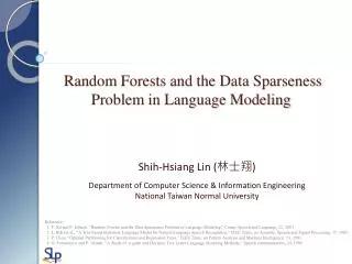
Random Forests for Language Modeling
Random Forests for Language Modeling. Peng Xu and Frederick Jelinek IPAM: January 24, 2006. What Is a Language Model?. A probability distribution over word sequences Based on conditional probability distributions: probability of a word given its history (past words). A. W*.

Random Forests for Language Modeling
E N D
Presentation Transcript
Random Forests for Language Modeling Peng Xu and Frederick Jelinek IPAM: January 24, 2006 CLSP, The Johns Hopkins University
What Is a Language Model? • A probability distribution over word sequences • Based on conditional probability distributions: probability of a word given its history (past words) CLSP, The Johns Hopkins University
A W* • Source-channel model W A What Is a Language Model for? • Speech recognition CLSP, The Johns Hopkins University
n-gram Language Models • A simple yet powerful solution to LM • (n-1) items in history: n-gram model • Maximum Likelihood (ML) estimate: • Sparseness Problem: training and test mismatch, most n-grams are never seen; need for smoothing CLSP, The Johns Hopkins University
Sparseness Problem Example: Upenn Treebank portion of WSJ, 1 million words training data, 82 thousand words test data, 10-thousand-word open vocabulary Sparseness makes language modeling a difficult regression problem: an n-gram model needs at least |V|n words to cover all n-grams CLSP, The Johns Hopkins University
More Data • More data solution to data sparseness • The web has “everything”: web data is noisy. • The web does NOT have everything: language models using web data still have data sparseness problem. • [Zhu & Rosenfeld, 2001] In 24 random web news sentences, 46 out of 453 trigrams were not covered by Altavista. • In domain training data is not always easy to get. CLSP, The Johns Hopkins University
Dealing With Sparseness in n-gram • Smoothing: take out some probability mass from seen n-grams and distribute among unseen n-grams • Interpolated Kneser-Ney: consistently the best performance [Chen & Goodman, 1998] CLSP, The Johns Hopkins University
Our Approach • Extend the appealing idea of history to clustering via decision trees. • Overcome problems in decision tree construction … by using Random Forests! CLSP, The Johns Hopkins University
Decision Tree Language Models • Decision trees: equivalence classification of histories • Each leaf is specified by the answers to a series of questions (posed to “history”) which lead to the leaf from the root. • Each leaf corresponds to a subset of the histories. Thus histories are partitioned (i.e.,classified). CLSP, The Johns Hopkins University
{ab,ac,bc,bb,ad} a:3 b:2 {ab,ac,ad} a:3 b:0 {bc,bb} a:0 b:2 Decision Tree Language Models: An Example Training data: aba, aca, bcb, bbb, ada New event ‘cba’ in test: Stuck! Is the first word in {a}? Is the first word in {b}? New event ‘adb’ in test New event ‘bdb’ in test CLSP, The Johns Hopkins University
Decision Tree Language Models: An Example • Example: trigrams (w-2,w-1,w0) • Questions about positions: “Is w-i2S?” and “Is w-i2Sc?” There are two history positions for trigram. • Each pair, S and Sc, defines a possible split of a node, and therefore, training data. • S and Sc are complements with respect to training data • A node gets less data than its ancestors. • (S, Sc) are obtained by an exchange algorithm. CLSP, The Johns Hopkins University
Construction of Decision Trees • Data Driven: decision trees are constructed on the basis of training data • The construction requires: • The set of possible questions • A criterion evaluating the desirability of questions • A construction stopping rule or post-pruning rule CLSP, The Johns Hopkins University
Construction of Decision Trees: Our Approach • Grow a decision tree until maximum depth using training data • Use training data likelihood to evaluate questions • Perform no smoothing during growing • Prune fully grown decision tree to maximize heldout data likelihood • Incorporate KN smoothing during pruning CLSP, The Johns Hopkins University
Smoothing Decision Trees • Using similar ideas as interpolated Kneser-Ney smoothing: • Note: • All histories in one node are not smoothed in the same way. • Only leaves are used as equivalence classes. CLSP, The Johns Hopkins University
Problems with Decision Trees • Training data fragmentation: • As tree is developed, the questions are selected on the basis of less and less data. • Lack of optimality: • The exchange algorithm is a greedy algorithm. • So is the tree growing algorithm • Overtraining and undertraining: • Deep trees: fit the training data well, will not generalize well to new test data. • Shallow trees: not sufficiently refined. CLSP, The Johns Hopkins University
Amelioration: Random Forests • Breiman applied the idea of random forests to relatively small problems. [Breiman 2001] • Using different random samples of data and randomly chosen subsets of questions, construct K decision trees. • Apply test datum x to all the different decision trees. • Produce classes y1,y2,…,yK. • Accept plurality decision: CLSP, The Johns Hopkins University
Example of a Random Forest T1 T2 T3 a a a a a a An example x will be classified as a according to this random forest. CLSP, The Johns Hopkins University
Random Forests for Language Modeling • Two kinds of randomness: • Selection of positions to ask about • Alternatives: position 1 or 2 or the better of the two. • Random initialization of the exchange algorithm • 100 decision trees: ithtree estimates • PDT(i)(w0|w-2,w-1) • The final estimate is the average of all trees CLSP, The Johns Hopkins University
Experiments • Perplexity (PPL): • UPenn Treebank part of WSJ: about 1 million words for training and heldout (90%/10%), 82 thousand words for test CLSP, The Johns Hopkins University
Experiments: trigram Baseline: KN-trigram No randomization: DT-trigram 100 random DTs: RF-trigram CLSP, The Johns Hopkins University
Experiments: Aggregating • Considerable improvement already with 10 trees! CLSP, The Johns Hopkins University
Experiments: Analysis • seen event: • KN-trigram: in training data • DT-trigram: in training data Analyze test data events by number of times seen in 100 DTs CLSP, The Johns Hopkins University
Experiments: Stability PPL results of different realizations varies, but differences are small. CLSP, The Johns Hopkins University
Aggregation: • Weighted average: Estimate weights so as to maximize heldout data log-likelihood Experiments: Aggregation v.s. Interpolation CLSP, The Johns Hopkins University
Optimal interpolation gains almost nothing! Experiments: Aggregation v.s. Interpolation CLSP, The Johns Hopkins University
Experiments: High Order n-grams Models • Baseline: KN n-gram • 100 random DTs: RF n-gram CLSP, The Johns Hopkins University
Using Random Forests to Other Models: SLM • Structured Language Model (SLM): [Chelba & Jelinek, 2000] • Approximation: use tree triples CLSP, The Johns Hopkins University
Speech Recognition Experiments (I) • Word Error Rate (WER) by N-best Rescoring: • WSJ text: 20 or 40 million words training • WSJ DARPA’93 HUB1 test data: 213 utterances, 3446 words • N-best rescoring: baseline WER is 13.7% • N-best lists were generated by a trigram baseline using Katz backoff smoothing. • The baseline trigram used 40 million words for training. • Oracle error rate is around 6%. CLSP, The Johns Hopkins University
Speech Recognition Experiments (I) Baseline: KN smoothing 100 random DTs for RF 3-gram 100 random DTs for the PREDICTOR in SLM Approximation in SLM CLSP, The Johns Hopkins University
Speech Recognition Experiments (II) • Word Error Rate by Lattice Rescoring • IBM 2004 Conversational Telephony System for Rich Transcription: 1st place in RT-04 evaluation • Fisher data: 22 million words • WEB data: 525 million words, using frequent Fisher n-grams as queries • Other data: Switchboard, Broadcast News, etc. • Lattice language model: 4-gram with interpolated Kneser-Ney smoothing, pruned to have 3.2 million unique n-grams, WER is 14.4% • Test set: DEV04, 37,834 words CLSP, The Johns Hopkins University
Speech Recognition Experiments (II) Baseline: KN 4-gram 110 random DTs for EB-RF 4-gram Sampling data without replacement Fisher and WEB models are interpolated CLSP, The Johns Hopkins University
Practical Limitations of the RF Approach • Memory: • Decision tree construction uses much more memory. • Little performance gain when training data is really large. • Because we have 100 trees, the final model becomes too large to fit into memory. • Effective language model compression or pruning remains an open question. CLSP, The Johns Hopkins University
Conclusions: Random Forests New RF language modeling approach More general LM: RF DT n-gram Randomized history clustering Good generalization: better n-gram coverage, less biased to training data Extension of Brieman’s random forests for data sparseness problem CLSP, The Johns Hopkins University
Conclusions: Random Forests • Improvements in perplexity and/or word error rate over interpolated Kneser-Ney smoothing for different models: • n-gram (up to n=6) • Class-based trigram • Structured Language Model • Significant improvements in the best performing large vocabulary conversational telephony speech recognition system CLSP, The Johns Hopkins University

