Download
1 / 53
540 likes | 1.2k Views
3 Introduction to Mass Transfer. Overview. Thermodynamics heat and mass transfer chemical reaction rate theory(chemical kinetics). Rudiments of Mass Transfer. Open a bottle of perfume in the center of a room---mass transfer Molecular processes(e.g., collisions in an ideal gas)

E N D
Overview • Thermodynamics • heat and mass transfer • chemical reaction rate theory(chemical kinetics)
Rudiments of Mass Transfer • Open a bottle of perfume in the center of a room---mass transfer • Molecular processes(e.g., collisions in an ideal gas) • turbulent processes.
Mass Transfer Rate Laws • Fick’s law of Diffusion • one dimension: Mass flow of species A per unit area Mass flow of species A associated with bulk flow per unit area Mass flow of species A associated with molecular diffusion per unit area
The mass flux is defined as the mass flowrate of species A per unit area perpendicular to the flow: • The units are kg/s-m2 • DAB is a property of the mixture and has units of m2/s, the binary diffusivity.
It means that species A is transported by two means: the first term on the right-hand-side representing the transported of A resulting from the bulk motion of the fluid, and the second term representing the diffusion of A superimposed on the bulk flow.
In the abseence of diffusion, we obtain the obvious result that • where is the mixture mass flux. The diffusion flux adds an additional component to the flux of A:
An analogy between the diffusion of mass and the diffusion of heat (conduction) can be drawn by comparing Fourier’s law of conduction:
The more general expression • where the bold symbols represent vector quantities. In many instants, the molar form of the above equation is useful:
Where is the molar flux(kmol/s-m2) of species A, xA is the mole fraction, and c is the mixture molar concentration(kmolmix/m3) • The meanings of bulk flow and diffusion flux become clearer if we express the total mass flux for a binary mixture as the sum of the mass flux of species A and the mass flux of species B:
Mixture mass flux Speies A mass flux Species B mass flux
For one dimension: • or
For a binary mixture, YA+YB=1, thus, Diffusional flux of species A Diffusional flux of species B
This is called ordinary diffusion. • Not binary mixture; • thermal diffusion • pressure diffusion.
Molecular basis of Diffusion • Kinetic theory of gases: Consider a stationary (no bulk flow) plane layer of a binary gas mixture consisting of rigid, nonattracting molecules in which the molecular mass of each species A and B is essential equal. A concentration(mass-fraction) gradient exists in the gas layer in the x-direction and is sufficiently small that the mass-fraction distribution can be considered linear over a distance of a few molecular mean free paths, , as illustrated in Fig 3.1
Where kB is Boltzmann’s constant; • mA the mass of a single A molecular, • nA/V is the number of A molecular per unit volume, • ntot/V is the total number of molecules per unit volume • is the diameter of both A and B molecules.
Assuming no bulk flow for simplicity, the net flux of A molecules at the x-plane is the difference between the flux of A molecules in the positive x-direction and the flux of A molecules in the negative x-direction: • which, when expressed in terms of the collision frequency, becomes
We can use the definition of density • (mtot/Vtot) to relate ZA”to the mass fraction of A molecules:
Substituting the above Equation into the early one, and treating the mixture density and mean molecular speeds as constants yields
With our assumption of a linear concentration distribution • Solving the above equation for the concentration difference and substituting into equation 3.14, we obtain our final result:
Comparing the above equation with the first equation, we define the binary diffusivity DAB as
Using the definitions of the mean molecular speed and mean free path, together with the ideal-gas equation of state PV=nkBT, the temperature and pressure dependence of DAB can easily be determined • or
Thus, we see that the diffusivity depends strongly on temperature( to the 3/2 power) and inversely with pressure. The mass flux of species A, however, depends on the product DAB,which has a square-root temperature dependence and is independent of pressure: • In many simplified analyses of combustion processes, the weak temperature dependence is neglected and D is treated as a constant.
Comparison with Heat Conduction • To see clearly the relationship between mass and heat transfer, we now apply kinetic theory to the transport of energy. We assume a homogeneous gas consisting of rigid nonattracting molecules in which a temperature gradient exists. Again, the gradient is sufficiently small that the temperature distribution is essentially linear over several mean free paths, as illustrated in Fig. 3.2.
The mean molecular speed and mean free path have the same definitions as given in Eqns. 3.10a and 3.10c, respectively; however, the molecular collision frequency of interest is now based on the total number density of molecules, ntot/V, i.e.,
In our no-interaction-at-a-distance hard-sphere model of the gas, the only energy storage mode is molesular translational, i.e., kinetic, energy. We write an energy balance at the x-direction is the difference between the kinetic energy flux associated with molecules traveling from x-a to x and those traveling form x+a to x
Since the mean kinetic energy of a molecule is given by • the heat flux can be related to the temperature as
The temperature difference in Eqn 3.22 relates to the temperature gradient following the same form as Eqn. 3.15 i.e., • Substituting difference in Eqn. 3.22 employing the definition of Z” and a, we obtain our final result for the heat flux:
Comparing the above with Fourier’s law of heat conduction(Eqn. 3.4), we can identify the thermal conductivity k as • Expressed in terms of T and molecular mass and size, the thermal conductivity is
The thermal conductivity is thus proportional to the square-root of temperature, • as is the DAB product. For real gases, the true temperature dependence is greater.
Species Conservation • Consider the one-dimensional control volume of Fig. 3.3, a plane layer x thick.
The net rate of increase in the mass of A within the control volume relates to the mass fluxes and reatction rate as follows: Mass flow of A into the control volume Rates of increase of mass of A within control volume Mass flow of A out of the control volume Mass prodution rate of species A by chemical reaction
is the mass production rate of species A per unit volume(kgA/m3-s). In Chapter 5, we specifically deal with how to determine . Recognizing that the mass of A within the control volume is mA,cv=Yamcv=YAVcv andthat the volume Vcv=Ax, Eqn. 3.28 can be written:
Dividing through by Ax and taking the limit as x0, Eqn. 3.29 becomes
Or, for the case of steady flow where • Equation 3.31 is the steady-flow, one-dimensional form of species conservation for a binary gas mixture, assuming species diffusion occurs only as a result of concentration gradients; i.e., only ordinary diffusion is considered. For the multidimensional case, Eqn. 3.31 can be generalized as
Net rate of production of species A by chemical reaction, per unit volume Net flow of species A out of control volume, per unit volume
Some application • The stefan Problem: • Consider liquid A, maintained at a fixed height in a glass cylinder as illustrated in Fig. 3.4.
Mathematically, the overall conservation of mass for this system can be expressed as • Since =0, then
Equation 3.1 now becomes: • Rearranging and separating variables, we obtain
Assuming the product DAB to be constant, Eqn. 3.36 can be integrated to yield • where C is the constant of integration. With the boundary condition:
We eliminate C and obtain the following mass-fraction distribution after removing the logarithm by exponentiation:
The mass flux of A, , can be found by letting YA(x=L)=YA,∞ in Eqn. 3.39. Thus,
From the above equation, we see that the mass flux is directly proportional to the product of the density and the mass diffusivity and inversely proportional to the length, L. Larger diffusivities thus produce larger mass fluxes. • To see the effects of the concentrations at the interface and at the top of the varying YA,i, the interface mass fraction, from zero to unity.