Understanding V1 --- Saliency map and pre-attentive segmentation

1. Understanding V1 --- Saliency map and pre-attentive segmentation Li Zhaoping University College London, Psychology www.gatsby.ucl.ac.uk/~zhaoping Lecture 2, at EU Advanced Course in Computational Neuroscience, Arcachon, France, Aug. 2006 Reading materials at www.gatsby.ucl.ac.uk/~zhaoping/ZhaopingNReview2006.pdf

2. Part 1: Explain & predict ? V1 outputs as simulated by a V1 model Visual saliencies in visual search and segmentation tasks Part 2: Psychophysical tests of the predictions of the V1 theory on the lack of individual feature maps and thus the lack of their summation to the final master map. Contrasting with previous theories of visual saliency. Outline A theory --- a saliency map in the primary visual cortex A computer vision motivation Testing the V1 theory

3. First, the theory A saliency map in primary visual cortex “A saliency map in primary visual cortex”, in Trends in Cognitive Sciences Vol 6, No. 1, page 9-16, 2002,

4. Contextual influences, and their confusing role: Weak suppression facilitation Strong suppression suppression What is in V1? Classical receptive fields: --- bar and edge detectors or filters, too small for global visual tasks. Horizontal intra-cortical connections observed as neural substrates

5. Larger receptive fields, much affected by visual attention. V2, V3, V4, IT, MT, PP etc. V1 Small receptive fields, limited effects from visual attention LGN retina Where is V1 in visual processing? V1 had traditionally been viewed as a lower visual area, as contributing little to complex visual phenomena. But, V1 is the largest visual area in the brain --- a hint towards my proposed role for V1.

6. Feature search Conjunction search Fast, parallel, pre-attentive, effortless, pops out Slow, serial, effortful, needs attention, does not pop out Psychophysical observations on visual saliency

7. A scalar map signaling saliency regardless of features Master saliency map in which cortical area? Not in V1 Color feature maps orientation feature maps Other: motion, depth, etc. red green green Feature maps in V2, V3, V4, V? blue blue Visual stimuli Previous views on saliency map(since 1970s --- Treisman, Julesz, Koch, Ullman, Wolfe, Mueller, Itti etc) A saliency map serves to select stimuli for further processing

8. Feature maps Master map Horizontal feature map Vertical feature map Explaining faster feature search: Feature search stimulus

9. Master map Feature maps vertical horizontal blue red Explaining slower conjunction search: Conjunction search stimulus

10. Traditional views on V1 Previous views on saliency map motion Master map Low level vision, non-complex visual phenomena Features maps etc blue Visual stimuli V1 physiology Saliency psychophysics Receptive fields and contextual influences

11. My proposal Firing rates of the V1’s output cells signal saliency regardless of feature tuning of the cells. V1 physiology Saliency psychophysics Receptive fields and contextual influences V1’s receptive fields and contextual influences are mechanisms to produce a saliency map from visual inputs Details in Zhaoping Li, “A saliency map in primary visual cortex”, in Trends in Cognitive Sciences Vol 6, No. 1, page 9-16, 2002,

12. Saliency from bottom-up factors only. Higher visual Areas Top-down Feedback disabled Saliency map Superior culliculus V1’s output as saliency map is viewed under the idealization of the top-down feedback to V1 being disabled, e.g., shortly after visual exposure or under anesthesia. V1 V1 producing a saliency map does not preclude it contributing to other visual functions such as object recognition.

13. More details Saliency outputs from V1 by cells’ firing rates (as universal currency for saliency) Transforming contrasts to saliencies by contextual influences V1 Conjunctive cells exist in V1 Contrast inputs to V1 Visual stimuli This theory requires: No separate feature maps, nor any summations of them V1 cells’ firing rates signal saliencies, despite their feature tuning Strongest response to any visual location signals its saliency

14. 1 $pike 3 $pike A motion tuned V1 cell A color tuned V1 cell Attention auctioned here, no discrimination between your feature preferences, only spikes count! Hmm… I am feature blind anyway Capitalist… he only cares about money!!! 2 $pike An orientation tuned V1 cell See: Zhaoping Li, “A saliency map in primary visual cortex”, in Trends in Cognitive Sciences Vol 6, No. 1, page 9-16, 2002,

15. Implementing the saliency map in a V1 model Saliency output from V1 model Highlighting important image locations. V1 model A recurrent network with Intra-cortical Interactions that executes contextual influences Contrast input to V1

16. Second: A computer vision motivation The segmentation problem(must be addressed for object recognition) To group image pixels belonging to one object Dilemma: Segmentation presumes recognition recognition presumes segmentation.

17. The usual approach: segmentation with (by) classification (1) image feature classification (2) Compare features to segment Problem: boundary precision vs. feature precision. To start: focusing on region segmentation A region can be characterized by its smoothness regularities, average luminance, and many more descriptions. Define segmentation as locating the border between regions. Dilemma: segmentation vs. classification

18. In biological vision: recognition (classification) is neither necessary nor sufficient for segmentation

19. Attentive: effortful, slow Pre-attentive and attentive segmentations -- very different. Pre-attentive: effortless, popout

20. Homogeneous input (one region) Inhomogeneous input (Two regions) My proposal:Pre-attentive segmentation without classification Principle: Detecting the boundaries by detecting translation invariance breaking in inputs via V1 mechanisms of contextual influences. Separating A from B without knowing what A and B are

21. Explain & predict? Test 1: Saliencies in visual search and segmentation tasks Outputs from a V1 A software V1 born 8 years ago Testing the V1 saliency map --- 1 Theory statement 1: Strongest V1 outputs at each location signal saliency

22. V1 outputs Contextual influences V1 units and initial responses Sampled by the receptive fields Designed such that the model agrees with physiology and produces desired behavior. Original image Schematics of how the model works

23. Recurrent dynamics dx i/dt = -xi + Jij g(xj) – g(yj) + Ii dy i/dt = -yi+ W ijg(xj) V1 model Intra-cortical Interactions The behavior of the network is ensured by computationally designing the recurrent connection weights, using dynamic system theory.

24. Conditions on the intra-cortical interactions. Outputs Inputs Highlight boundary Enhance contour No symmetry breaking (hallucination) No gross extension Design techniques: mean field analysis, stability analysis. Computation desired constraints the network architecture, connections, and dynamics. Network oscillation is one of the dynamic consequences.

25. Make sure that the model can produce the usual contextual influences Iso-orientation suppression Random surround less suppression Cross orientation least suppression Co-linear facilitation Single bar Input output

26. Proposal: V1 produces a saliency map S=0.2, Z=1.0 S=0.4, Z=7 Z=-1.3 S=0.12, Z=1.7 S=0.22 Histogram of all responses S regardless of features Pop-out Saliency map s Z = (S-S)/σ --- z score, measuring saliencies of items  Original input V1 response S

27. input V1 output Target = + Feature search --- pop out Z=7 Target= Conjunction search --- serial search Z= - 0.9 The V1 saliency map agrees with visual search behavior.

28. Prediction:bias in the perceptual estimation of the location of the texture boundary. Texture segmentation simulation results --- quantitative agreement with psychophysics (Nothdurft’s data) V1 model input V1 model output

29. Segmentation without classification V1 model inputs More complex patterns V1 model output highlights

30. input V1 output Target = + Feature search --- pop out Z=7 Target lacking a feature Target = Z=0.8 A trivial example of search asymmetry

31. Psychophysical definition: enables pop-out basic feature new What defines a basic feature? Computational or mechanistic definition: two neural components or substrates required for basic features: (1) Tuning of the cell receptive field to the feature (2) Tuning of the horizontal connections to the feature --- the horizontal connections are selective to that optimal feature, e.g.,orientation, of the pre- and post- synaptic cells.

32. There should be a continuum from pop-out to serial searches The ease of search is measured by a graded number : z score Treisman’s original Feature Integration Theory may be seen as the discrete idealization of the search process.

33. Saliency measure: Z = (S- S)/σ Influence of the background homogeneities (cf. Duncan & Humphreys, and Rubinstein & Sagi.) σ increases with the background in-homogeneity. Hence, homogeneous background makes target more salient.

34. Inputs V1 outputs Same target, different backgrounds Distractors irregularly placed Target= Z=0.22 The easiest search Target= Distractors dissimilar to each other Z=0.25 Homogeneous background, identical distractors regularly placed Target= Z=3.4 Explains spatial configuration and distractor effects.

35. Z=-0.63, next to target, z=0.68 Distractors irregularly placed Neighbors attract attention to target. Target= Homogeneous background, identical distractors regularly placed Z=-0.83, next to target, z=3.7 Target= Another example of background regularity effect Input Output

36. Open vs. closed parallel vs. divergent long vs. short curved vs. straight elipse vs. circle Z=0.41 Z= -1.4 Z= -0.06 Z= 0.3 Z= 0.7 Z=9.7 Z= 2.8 Z= 1.8 Z= 1.07 Z= 1.12 More severe test of the saliency map theory by using subtler saliency phenomena --- search asymmetries (Treisman)

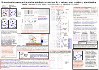
37. Conjunction search revisited Output Input Some conjunction searches are easy e.g.: Conjunctions of motion and form (orientation) --- McLeod, Driver, Crisp 1988) e.g., Conjunctions of depth and motion or color --- Nakayama and Silverman 1986. Why?

38. Recall the two neural components necessary for a basic feature (1) Tuning of the receptive field (CRF) (2) Tuning of the horizontal connections For a conjunction to be basic and pop-out: (1) Simultaneous or conjunctive tunings of the V1 cells to both feature dimensions (e.g., orientation & motion, orientation and depth, but not orientation and orientation) (2) Simultaneous or conjunctive tunings of the horizontal connections to the optimal features in both feature dimensions of the pre- and post- synaptic cells

39. Predicting from psychophysics to V1 anatomy Since conjunctions of motion and orientation, and depth and motion or color, pop-out The horizontal connections must be selective simultaneously to both orientation & motion, and to both depth and motion (or color)--- can be tested Note that it is already know that V1 cells can be simultaneously tuned to orientation, motion direction, depth (and even color sometimes)

40. Color-orientation conjunction? Prediction: Color-orientation conjunction search can be made easier by adjusting the scale and/or density of the stimuli, since V1 cells conjunctively tuned to both orientation and color are mainly tuned to a specific spatial frequency band. Stimuli for a conjunction search for target Response from a model without conjunction cells Response from a model with conjunction cells

41. Single feature searches Double feature search --- opposite of conjunction search Responses to target from 3 cell types: (1) orientation tuned cells tuned to vertical (2) color tuned cells tuned to red (3) conjunctively tuned cells tuned to red-vertical The most responsive of them should signal the target saliency. Let (1) and (2) determine eases in single searches. Existence of (3) makes double feature search possibly easier. How easy is double feature compared to single feature searches? Explains Nothdurft (2000) data: orientation-motion double feature search is easier than orientation-color double feature search.

42. Test 2: (Joint work with Keith May) Test predictions from “strongest response” rule, contrast with predictions fromfeature map summation rule from previous theories/models. Testing the V1 saliency map --- 2 Theory statement 2: No separate feature maps, nor any summations of them, are needed. Simply, the strongest response at a location signal saliency. Contrast with previous theories: feature maps sum to get the master saliency map

43. No separate feature maps, strongest response rule regardless of feature tunings. Approximately equivalent to Separate feature maps, maximize over feature maps. Then: Previous theories The V1 theory vs. Max rule Summation rule To compare “strongest response rule” with “feature map summation rule” --- put the two in the same footing: When each cell signals only one feature, i.e., when there are no cells tuned to more than one feature (conjunctively tuned cells) When the interaction between cells tuned to different features are approximated as zero.

44. (Summed or max-ed) Combined map Separate feature maps Separate activity maps Consider texture segmentation tasks Stimulus No difference between two theories.

45. Stimulus Combined map Separate feature maps Separate activity maps sum max + = Predicts easier segmentation than either component Predicts segmentation of the same ease as the easiest component

46. Task: subject answer whether the texture border is left or right Error rates Reaction time (ms) Test: measure reaction times in segmentations:

47. Data from five subjects Reaction times (ms) AJ AL KM LZ AI Error rates

48. Not a floor effect --- same observation on more difficult texture segmentations Subject LZ Error rates Reaction time (ms)

49. Feature activation maps Partial combinations of activation maps Combined maps Feature maps sum max Stimulus = + Predicts easy segmentation Homogeneous activations Predicts difficult segmentation

50. Test: measure reaction times in same segmentation tasks: AI Error rates Reaction time (ms)