Download
1 / 35
350 likes | 394 Views
Explore Bayesian statistical methods in particle physics and their role in data analysis, fitting problems, limits setting, and more. Understand how probability, uncertainties, and theories come into play. Learn about the interpretation of probability, Bayes' theorem, and the difference between frequentist and Bayesian statistics.

E N D
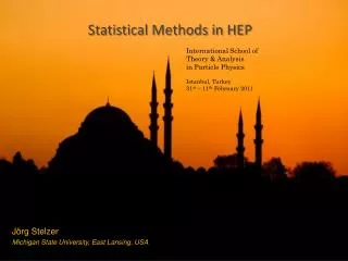
Statistical Methods in Particle PhysicsLecture 1: Bayesian methods SUSSP65 St Andrews 16–29 August 2009 Glen Cowan Physics Department Royal Holloway, University of London g.cowan@rhul.ac.uk www.pp.rhul.ac.uk/~cowan SUSSP65, St Andrews, 16-29 August 2009 / Statistical Methods 1
Outline Lecture #1: An introduction to Bayesian statistical methods Role of probability in data analysis (Frequentist, Bayesian) A simple fitting problem : Frequentist vs. Bayesian solution Bayesian computation, Markov Chain Monte Carlo Lecture #2: Setting limits, making a discovery Frequentist vs Bayesian approach, treatment of systematic uncertainties Lecture #3: Multivariate methods for HEP Event selection as a statistical test Neyman-Pearson lemma and likelihood ratio test Some multivariate classifiers: NN, BDT, SVM, ... SUSSP65, St Andrews, 16-29 August 2009 / Statistical Methods 1
Data analysis in particle physics Observe events of a certain type Measure characteristics of each event (particle momenta, number of muons, energy of jets,...) Theories (e.g. SM) predict distributions of these properties up to free parameters, e.g., a, GF, MZ, as, mH, ... Some tasks of data analysis: Estimate (measure) the parameters; Quantify the uncertainty of the parameter estimates; Test the extent to which the predictions of a theory are in agreement with the data (→presence of New Physics?) SUSSP65, St Andrews, 16-29 August 2009 / Statistical Methods 1
Dealing with uncertainty In particle physics there are various elements of uncertainty: theory is not deterministic quantum mechanics random measurement errors present even without quantum effects things we could know in principle but don’t e.g. from limitations of cost, time, ... We can quantify the uncertainty usingPROBABILITY SUSSP65, St Andrews, 16-29 August 2009 / Statistical Methods 1
A definition of probability Consider a set S with subsets A, B, ... Kolmogorov axioms (1933) Also define conditional probability: SUSSP65, St Andrews, 16-29 August 2009 / Statistical Methods 1
Interpretation of probability I. Relative frequency A, B, ... are outcomes of a repeatable experiment cf. quantum mechanics, particle scattering, radioactive decay... II. Subjective probability A, B, ... are hypotheses (statements that are true or false) • Both interpretations consistent with Kolmogorov axioms. • In particle physics frequency interpretation often most useful, but subjective probability can provide more natural treatment of non-repeatable phenomena: systematic uncertainties, probability that Higgs boson exists,... SUSSP65, St Andrews, 16-29 August 2009 / Statistical Methods 1
Bayes’ theorem From the definition of conditional probability we have and , so but Bayes’ theorem First published (posthumously) by the Reverend Thomas Bayes (1702−1761) An essay towards solving a problem in the doctrine of chances, Philos. Trans. R. Soc. 53 (1763) 370; reprinted in Biometrika, 45 (1958) 293. SUSSP65, St Andrews, 16-29 August 2009 / Statistical Methods 1
B The law of total probability Consider a subset B of the sample space S, S divided into disjoint subsets Ai such that [i Ai = S, Ai B∩ Ai → → law of total probability → Bayes’ theorem becomes SUSSP65, St Andrews, 16-29 August 2009 / Statistical Methods 1
Frequentist Statistics − general philosophy In frequentist statistics, probabilities are associated only with the data, i.e., outcomes of repeatable observations. Probability = limiting frequency Probabilities such as P (Higgs boson exists), P (0.117 < as < 0.121), etc. are either 0 or 1, but we don’t know which. The tools of frequentist statistics tell us what to expect, under the assumption of certain probabilities, about hypothetical repeated observations. The preferred theories (models, hypotheses, ...) are those for which our observations would be considered ‘usual’. SUSSP65, St Andrews, 16-29 August 2009 / Statistical Methods 1
Bayesian Statistics − general philosophy In Bayesian statistics, interpretation of probability extended to degree of belief (subjective probability). Use this for hypotheses: probability of the data assuming hypothesis H (the likelihood) prior probability, i.e., before seeing the data posterior probability, i.e., after seeing the data normalization involves sum over all possible hypotheses Bayesian methods can provide more natural treatment of non- repeatable phenomena: systematic uncertainties, probability that Higgs boson exists,... No golden rule for priors (“if-then” character of Bayes’ thm.) SUSSP65, St Andrews, 16-29 August 2009 / Statistical Methods 1
Statistical vs. systematic errors Statistical errors: How much would the result fluctuate upon repetition of the measurement? Implies some set of assumptions to define probability of outcome of the measurement. Systematic errors: What is the uncertainty in my result due to uncertainty in my assumptions, e.g., model (theoretical) uncertainty; modeling of measurement apparatus. Usually taken to mean the sources of error do not vary upon repetition of the measurement. Often result from uncertain value of calibration constants, efficiencies, etc. SUSSP65, St Andrews, 16-29 August 2009 / Statistical Methods 1
Systematic errors and nuisance parameters Model prediction (including e.g. detector effects) never same as "true prediction" of the theory: model: y truth: x Model can be made to approximate better the truth by including more free parameters. systematic uncertainty ↔ nuisance parameters SUSSP65, St Andrews, 16-29 August 2009 / Statistical Methods 1
Example: fitting a straight line Data: Model: measured yi independent, Gaussian: assume xi and si known. Goal: estimate q0 (don’t care about q1). SUSSP65, St Andrews, 16-29 August 2009 / Statistical Methods 1
Frequentist approach with q1 known a priori For Gaussian yi, ML same as LS Minimize c2→estimator Come up one unit from to find SUSSP65, St Andrews, 16-29 August 2009 / Statistical Methods 1
Frequentist approach with both q0 and q1 unknown Standard deviations from tangent lines to contour Correlation between causes errors to increase. SUSSP65, St Andrews, 16-29 August 2009 / Statistical Methods 1
The profile likelihood The ‘tangent plane’ method is a special case of using the profile likelihood: is found by maximizing L (q0, q1) for each q0. Equivalently use The interval obtained from is the same as what is obtained from the tangents to Well known in HEP as the ‘MINOS’ method in MINUIT. Profile likelihood is one of several ‘pseudo-likelihoods’ used in problems with nuisance parameters. See e.g. talk by Rolke at PHYSTAT05. SUSSP65, St Andrews, 16-29 August 2009 / Statistical Methods 1
Frequentist case with a measurement t1 of q1 The information on q1 improves accuracy of SUSSP65, St Andrews, 16-29 August 2009 / Statistical Methods 1
The Bayesian approach In Bayesian statistics we can associate a probability with a hypothesis, e.g., a parameter value q. Interpret probability of q as ‘degree of belief’ (subjective). Need to start with ‘prior pdf’ p(q), this reflects degree of belief about q before doing the experiment. Our experiment has data x, → likelihood functionL(x|q). Bayes’ theorem tells how our beliefs should be updated in light of the data x: Posterior pdf p(q|x) contains all our knowledge about q. SUSSP65, St Andrews, 16-29 August 2009 / Statistical Methods 1
Bayesian method We need to associate prior probabilities with q0 and q1, e.g., reflects ‘prior ignorance’, in any case much broader than ←based on previous measurement Putting this into Bayes’ theorem gives: posterior likelihood prior SUSSP65, St Andrews, 16-29 August 2009 / Statistical Methods 1
Bayesian method (continued) We then integrate (marginalize) p(q0, q1 | x) to find p(q0 | x): In this example we can do the integral (rare). We find Usually need numerical methods (e.g. Markov Chain Monte Carlo) to do integral. SUSSP65, St Andrews, 16-29 August 2009 / Statistical Methods 1
Digression: marginalization with MCMC Bayesian computations involve integrals like often high dimensionality and impossible in closed form, also impossible with ‘normal’ acceptance-rejection Monte Carlo. Markov Chain Monte Carlo (MCMC) has revolutionized Bayesian computation. MCMC (e.g., Metropolis-Hastings algorithm) generates correlated sequence of random numbers: cannot use for many applications, e.g., detector MC; effective stat. error greater than if uncorrelated . Basic idea: sample multidimensional look, e.g., only at distribution of parameters of interest. SUSSP65, St Andrews, 16-29 August 2009 / Statistical Methods 1
Example: posterior pdf from MCMC Sample the posterior pdf from previous example with MCMC: Summarize pdf of parameter of interest with, e.g., mean, median, standard deviation, etc. Although numerical values of answer here same as in frequentist case, interpretation is different (sometimes unimportant?) SUSSP65, St Andrews, 16-29 August 2009 / Statistical Methods 1
MCMC basics: Metropolis-Hastings algorithm Goal: given an n-dimensional pdf generate a sequence of points Proposal density e.g. Gaussian centred about 1) Start at some point 2) Generate 3) Form Hastings test ratio 4) Generate move to proposed point 5) If else old point repeated 6) Iterate SUSSP65, St Andrews, 16-29 August 2009 / Statistical Methods 1
Metropolis-Hastings (continued) This rule produces a correlated sequence of points (note how each new point depends on the previous one). For our purposes this correlation is not fatal, but statistical errors larger than it would be with uncorrelated points. The proposal density can be (almost) anything, but choose so as to minimize autocorrelation. Often take proposal density symmetric: Test ratio is (Metropolis-Hastings): I.e. if the proposed step is to a point of higher , take it; if not, only take the step with probability If proposed step rejected, hop in place. SUSSP65, St Andrews, 16-29 August 2009 / Statistical Methods 1
Metropolis-Hastings caveats Actually one can only prove that the sequence of points follows the desired pdf in the limit where it runs forever. There may be a “burn-in” period where the sequence does not initially follow Unfortunately there are few useful theorems to tell us when the sequence has converged. Look at trace plots, autocorrelation. Check result with different proposal density. If you think it’s converged, try starting from a different point and see if the result is similar. SUSSP65, St Andrews, 16-29 August 2009 / Statistical Methods 1
Bayesian method with alternative priors Suppose we don’t have a previous measurement of q1 but rather, e.g., a theorist says it should be positive and not too much greater than 0.1 "or so", i.e., something like From this we obtain (numerically) the posterior pdf for q0: This summarizes all knowledge about q0. Look also at result from variety of priors. SUSSP65, St Andrews, 16-29 August 2009 / Statistical Methods 1
A more general fit (symbolic) Given measurements: and (usually) covariances: Predicted value: expectation value control variable parameters bias Often take: Minimize Equivalent to maximizing L() » e-2/2, i.e., least squares same as maximum likelihood using a Gaussian likelihood function. SUSSP65, St Andrews, 16-29 August 2009 / Statistical Methods 1
Its Bayesian equivalent Take Joint probability for all parameters and use Bayes’ theorem: To get desired probability for , integrate (marginalize) over b: →Posterior is Gaussian with mode same as least squares estimator, same as from 2 = 2min + 1. (Back where we started!) SUSSP65, St Andrews, 16-29 August 2009 / Statistical Methods 1
Alternative priors for systematic errors Gaussian prior for the bias b often not realistic, especially if one considers the "error on the error". Incorporating this can give a prior with longer tails: Represents ‘error on the error’; standard deviation of ps(s) is ss. b(b) b SUSSP65, St Andrews, 16-29 August 2009 / Statistical Methods 1
A simple test Suppose fit effectively averages four measurements. Take sys = stat = 0.1, uncorrelated. Case #1: data appear compatible Posterior p(|y): measurement p(|y) experiment Usually summarize posterior p(|y) with mode and standard deviation: SUSSP65, St Andrews, 16-29 August 2009 / Statistical Methods 1
Simple test with inconsistent data Case #2: there is an outlier Posterior p(|y): measurement p(|y) experiment →Bayesian fit less sensitive to outlier. (See also D'Agostini 1999; Dose & von der Linden 1999) SUSSP65, St Andrews, 16-29 August 2009 / Statistical Methods 1
Goodness-of-fit vs. size of error In LS fit, value of minimized 2 does not affect size of error on fitted parameter. In Bayesian analysis with non-Gaussian prior for systematics, a high 2 corresponds to a larger error (and vice versa). 2000 repetitions of experiment, s = 0.5, here no actual bias. posterior from least squares 2 SUSSP65, St Andrews, 16-29 August 2009 / Statistical Methods 1
Summary of lecture 1 The distinctive features of Bayesian statistics are: Subjective probability used for hypotheses (e.g. a parameter). Bayes' theorem relates the probability of data given H (the likelihood) to the posterior probability of H given data: Requires prior probability for H Bayesian methods often yield answers that are close (or identical) to those of frequentist statistics, albeit with different interpretation. This is not the case when the prior information is important relative to that contained in the data. SUSSP65, St Andrews, 16-29 August 2009 / Statistical Methods 1
Extra slides SUSSP65, St Andrews, 16-29 August 2009 / Statistical Methods 1
Some Bayesian references P. Gregory, Bayesian Logical Data Analysis for the Physical Sciences, CUP, 2005 D. Sivia, Data Analysis: a Bayesian Tutorial, OUP, 2006 S. Press, Subjective and Objective Bayesian Statistics: Principles, Models and Applications, 2nd ed., Wiley, 2003 A. O’Hagan, Kendall’s, Advanced Theory of Statistics, Vol. 2B, Bayesian Inference, Arnold Publishers, 1994 A. Gelman et al., Bayesian Data Analysis, 2nd ed., CRC, 2004 W. Bolstad, Introduction to Bayesian Statistics, Wiley, 2004 E.T. Jaynes, Probability Theory: the Logic of Science, CUP, 2003 SUSSP65, St Andrews, 16-29 August 2009 / Statistical Methods 1