FAUST Functional Analytic Unsupervised and Supervised data mining Technology Dr. William Perrizo
110 likes | 133 Views
This work involves clustering and classifying large datasets using vertically structured pTrees for efficient and effective data mining. Explore the evolution and challenges of working with big data.

FAUST Functional Analytic Unsupervised and Supervised data mining Technology Dr. William Perrizo
E N D
Presentation Transcript
FAUST Functional Analytic Unsupervised and Supervised data mining Technology Dr. William Perrizo University Distinguished Professor of Computer Science North Dakota State University, Fargo, ND William.perrizo@ndsu.edu visit Treeminer, Inc. 175 Admiral Cochrane Dr. Suite 300Annapolis, Maryland 21401240.389.0750 (T)301.528.6297 (F)info@treeminer.com
This work involves clustering and classification of very big datasets (so called "big data")using vertically structuring (pTrees) In a nutshell our techniques involve structuring the dataset into compressed vertical strips (bitslices) and processing across those vertical bitslices using logical operations. This is in contrast to the traditional method, that of structuring the data into horizontal records and then processing down those record. Thus, we do horizontal processing of vertical data (HPVD) rather than the traditional vertical processing of horizontal data (VPHD). We will take a much more detail look at the way we structure data and the way we process those structures a little later, but first, I want to talk about big data. How big is big data these days and how big will it get? An example.
The US Library of Congress is storing EVERY tweet that was sent since Twitter launched in 2006 Each tweet record contains fifty fields Let's assume a tweet record is 1000 bits in width The US LoC will record 172 Billion tweets from 500 million tweeters in 2013 alone. So let's estimate approximately 1 trillion tweets from 1 billion tweeters, to 1 billion tweetees from 2006 to 2016. As a full 3-dimensional matrix that's an undecillion=1030 matrix cells Even if only the sender is recorded, that's a 1000 excillion=1021.
Let’s look at how the definition of “big data” has evolved just over my work lifetime. I started as THE technician at the St. John’s University IBM 1620 Computer Center (circa 1964), I did the following: 1. I turned the 1620 switch on. 2. I waited for the ready light bulb to come on (~15 minutes) 3. I put the O/S punch card stack on the card reader (~4 in. high) 4. I put the FORTRAN compiler card stack on the reader (~3 in.) 5. I put the FORTRAN program card stack on the reader (~2 in.) 6. The 1620 produced an object code stack which I read in (~1 in 7. I read in the object stack and a 1964 big datastack (~40 in.) The 1st FORTRAN upgrade allowed for a “continue” card so that the data stack could be read in segments (and I could sit down).
How high would a 2013 big data stack of Hollerith punch cards reach? Let's be conservative and just assume an exabyte of data on punch cards How high is an exabyte on punch cards? We're being conservative because the US LoC full matrix of tweet data would be ~1030 bytes (and an exabyte is a mere 1018)
That exabyte stack of punch cards would reach JUPITER! So, in my work lifetime, "big data" has gone from 40 inches high all the way to Jupiter! What will happen to big data over my grandson, Will-the-2nd’s, lifetime?
Will-the-1st (that's me) has to deal with a stack of tweets that will reach Jupiter, but I will replace it, losslessly by 1000 extendable vertical pTrees and data mine across those 1000 horizontally. Will-the-2nd will have to deal with a stack of tweets that will reach the end of space, but he will replace it losslessly by 1000 extendable vertical pTrees and data mine across those 1000 horizontally. Will-the-3rd, will have to deal with a stack of tweets that will create new space, but he will replace it losslessly by 1000 extendable vertical pTrees and data mine across those 1000 horizontally. Will-the-3rd can use Will the-2nd's code (which is Will-the-1st's code). Will-the-3rd ‘s DATA WILL HAVE TO BE COMPRESSED and have to be VERTICALLY structured (I believe). Let's see how compressed vertical data structuring might be done.
predicate Trees = pTrees: slice by column (4 vertical structures). Vertical Data (pTrees) Traditional Vertical Processing of Horizontal Data (VPHD) e.g., find the number of occurences of 7 0 1 4 Using vertical pTreesfind number of occurences 7 0 1 4 T[A1] T[A2] T[A3] T[A4] T(A1 A2 A3 A4) 2 7 6 1 6 7 6 0 3 7 5 1 2 7 5 7 3 2 1 4 2 2 1 5 7 0 1 4 7 0 1 4 010 111 110 001 011 111 110 000 010 110 101 001 010 111 101 111 011 010 001 100 010 010 001 101 111 000 001 100 111 000 001 100 010 111 110 001 011 111 110 000 010 110 101 001 010 111 101 111 011 010 001 100 010 010 001 101 111 000 001 100 111 000 001 100 for Horizontally structured, record-oriented data, one scans vertically = pure1? true=1 pure1? false=0 T11 T12 T13 T21 T22 T23 T31 T32 T33 T41 T42 T43 0 1 0 1 1 1 1 1 0 0 0 1 0 1 1 1 1 1 1 1 0 0 0 0 0 1 0 1 1 0 1 0 1 0 0 1 0 1 0 1 1 1 1 0 1 1 1 1 0 1 1 0 1 0 0 0 1 1 0 0 0 1 0 0 1 0 0 0 1 1 0 1 1 1 1 0 0 0 0 0 1 1 0 0 1 1 1 0 0 0 0 0 1 1 0 0 pure1? false=0 pure1? false=0 pure1? false=0 0 0 0 1 0 01 0 1 0 1 0 1 1. Whole thing pure1? false 0 P11 P12 P13 P21 P22 P23 P31 P32 P33 P41 P42 P43 2. Left half pure1? false 0 P11 0 0 0 0 0 01 3. Right half pure1? false 0 0 0 0 0 1 0 0 10 01 0 0 0 1 0 0 0 0 0 0 0 1 01 10 0 0 0 0 1 0 0 0 0 1 0 0 0 0 0 0 0 0 0 0 0 1 0 0 0 1 0 0 ^ ^ ^ ^ ^ ^ ^ 0 0 1 0 1 4. Left half of rt half? false0 7 0 1 4 0 0 1 0 0 01 5. Rt half of right half? true1 0 *23 0 0 *22 =2 0 1 *21 *20 0 1 0 To count (7,0,1,4)s use 111000001100P11^P12^P13^P’21^P’22^P’23^P’31^P’32^P33^P41^P’42^P’43 = vertically slice off each bit position (12 vertical structures) then compress each bit slice into a treeusing a predicate (We will walk thru the compression of T11 into pTree, P11 ) =2 Base 10 Base 2 T11 0 0 0 0 0 0 1 1 Imagine an excillion records, not just 8 (We need speed!). Record truth of predicate: "purely 1-bits" in a tree, recursively on halves, until the half is pure. More typically, we compress strings of bits not single bits (eg, 64 bit strings or strides). P11 But it's pure0 so this branch ends
FAUST=Functional Analytic Unsupervised and Supervised data mining Technology CLUSTERing (unsupervised) Use functional gap analysis to find round clusters: • Initially let C = entire table, X, e.g., X≡{p1, ..., pf}, an image table of 15 pixels). • While cluster C, is insufficiently dense, find M = Mean(C) (or Vector_of_Medians?). • Pick a point fC (e.g., the furthest point fromM)and let fM denote the vector from f to M. • If count(C) / |fM|2 > DT (a DensityThreshold), C is complete, • else split C at each cutpoint P where there is a GT gap (GT=Gap Threshold) in the dot product values, C dot d≡fM/|fM| Speed? What if there are a trillion pixels (not just 15)? Interlocking horseshoes with an outlier 1 2 p2 p5 p1 3 p4 p6 p9 4 p3 p8 p7 5 pf pb 6 pe pc 7 pd pa 8 1 2 3 4 5 6 7 8 9 a b c d e f C2={p5}is complete (a singleton = outlier). C3={p6,pf} will split into {p6} and {pf} which are also outliers (details omitted) That leaves C1={p1,p2,p3,p4} and C4={p7,p8,p9,pa,pb,pc,pd,pe} still incomplete. C1 is complete ( density(C1)= ~4/22=1 > DT=.5 ?) Applying the algorithm to C4: In both cases those are probably the best "round" clusters (accurate?). All calculations can be done using pTrees (processing across the 8 pTrees regardless of the number of pixels.) 1 p1 p2 p7 2 p3 p5 p8 3 p4 p6 p9 4 pa 5 6 7 8 pf 9 pb a pc b pd pe c d e f 0 1 2 3 4 5 6 7 8 9 a b c d e f Finally, there are many variations of this algorithm (e.g. using M=vector_of_medians instead of the mean, which works better for finding outliers! M f M4 X x1 x2 p1 1 1 p2 3 1 p3 2 2 p4 3 3 p5 6 2 p6 9 3 p7 15 1 p8 14 2 p9 15 3 pa 13 4 pb 10 9 pc 11 10 pd 9 11 pe 11 11 pf 7 8 C1 C2 C3 C4 {pa} is an outlier. C2 splits into {p9}, {pb,pc,pd}, both complete. M1 M0 f f1=p3, C1 doesn't split (complete).
Finding FAUST gaps using pTree HPVD (Horizontal Process of Vertical Data) xofM 11 27 23 34 53 80 118 114 125 114 110 121 109 125 83 p6 0 0 0 0 0 1 1 1 1 1 1 1 1 1 1 p5 0 0 0 1 1 0 1 1 1 1 1 1 1 1 0 p4 0 1 1 0 1 1 1 1 1 1 0 1 0 1 1 p3 1 1 0 0 0 0 0 0 1 0 1 1 1 1 0 p2 0 0 1 0 1 0 1 0 1 0 1 0 1 1 0 p1 1 1 1 1 0 0 1 1 0 1 1 0 0 0 1 p0 1 1 1 0 1 0 0 0 1 0 0 1 1 1 1 p6' 1 1 1 1 1 0 0 0 0 0 0 0 0 0 0 p5' 1 1 1 0 0 1 0 0 0 0 0 0 0 0 1 p4' 1 0 0 1 0 0 0 0 0 0 1 0 1 0 0 p3' 0 0 1 1 1 1 1 1 0 1 0 0 0 0 1 p2' 1 1 0 1 0 1 0 1 0 1 0 1 0 0 1 p1' 0 0 0 0 1 1 0 0 1 0 0 1 1 1 0 p0' 0 0 0 1 0 1 1 1 0 1 1 0 0 0 0 X x1 x2 p1 1 1 p2 3 1 p3 2 2 p4 3 3 p5 6 2 p6 9 3 p7 15 1 p8 14 2 p9 15 3 pa 13 4 pb 10 9 pc 11 10 pd 9 11 pe 11 11 pf 7 8 OR between gap 2 and 3 for cluster C2={p5} [uncompressed] pTrees of xofM f=p1 GT=8=23. p5' 1 1 1 0 0 1 0 0 0 0 0 0 0 0 1 p4' 1 0 0 1 0 0 0 0 0 0 1 0 1 0 0 p6' 1 1 1 1 1 0 0 0 0 0 0 0 0 0 0 p5' 1 1 1 0 0 1 0 0 0 0 0 0 0 0 1 p3' 0 0 1 1 1 1 1 1 0 1 0 0 0 0 1 p5' 1 1 1 0 0 1 0 0 0 0 0 0 0 0 1 p4' 1 0 0 1 0 0 0 0 0 0 1 0 1 0 0 p3 1 1 0 0 0 0 0 0 1 0 1 1 1 1 0 p4 0 1 1 0 1 1 1 1 1 1 0 1 0 1 1 p5' 1 1 1 0 0 1 0 0 0 0 0 0 0 0 1 p3' 0 0 1 1 1 1 1 1 0 1 0 0 0 0 1 p3 1 1 0 0 0 0 0 0 1 0 1 1 1 1 0 p4 0 1 1 0 1 1 1 1 1 1 0 1 0 1 1 p6' 1 1 1 1 1 0 0 0 0 0 0 0 0 0 0 p5 0 0 0 1 1 0 1 1 1 1 1 1 1 1 0 p3' 0 0 1 1 1 1 1 1 0 1 0 0 0 0 1 p4' 1 0 0 1 0 0 0 0 0 0 1 0 1 0 0 p4' 1 0 0 1 0 0 0 0 0 0 1 0 1 0 0 p6' 1 1 1 1 1 0 0 0 0 0 0 0 0 0 0 p3 1 1 0 0 0 0 0 0 1 0 1 1 1 1 0 p5 0 0 0 1 1 0 1 1 1 1 1 1 1 1 0 p3' 0 0 1 1 1 1 1 1 0 1 0 0 0 0 1 p4 0 1 1 0 1 1 1 1 1 1 0 1 0 1 1 p5 0 0 0 1 1 0 1 1 1 1 1 1 1 1 0 p4 0 1 1 0 1 1 1 1 1 1 0 1 0 1 1 p5 0 0 0 1 1 0 1 1 1 1 1 1 1 1 0 p6' 1 1 1 1 1 0 0 0 0 0 0 0 0 0 0 p6' 1 1 1 1 1 0 0 0 0 0 0 0 0 0 0 p6' 1 1 1 1 1 0 0 0 0 0 0 0 0 0 0 p6' 1 1 1 1 1 0 0 0 0 0 0 0 0 0 0 p6' 1 1 1 1 1 0 0 0 0 0 0 0 0 0 0 p3 1 1 0 0 0 0 0 0 1 0 1 1 1 1 0 23gap: [40,47] = [010 1000, 010 1111] 23 gap: [0,7]= [000 0000, 000 0111], but since it is at the front, it doesn't separate clusters. 23gap: [56,63] = [011 1000, 011 1111] p6 0 0 0 0 0 1 1 1 1 1 1 1 1 1 1 p5' 1 1 1 0 0 1 0 0 0 0 0 0 0 0 1 p6 0 0 0 0 0 1 1 1 1 1 1 1 1 1 1 p5 0 0 0 1 1 0 1 1 1 1 1 1 1 1 0 p6 0 0 0 0 0 1 1 1 1 1 1 1 1 1 1 p5 0 0 0 1 1 0 1 1 1 1 1 1 1 1 0 p5 0 0 0 1 1 0 1 1 1 1 1 1 1 1 0 p5' 1 1 1 0 0 1 0 0 0 0 0 0 0 0 1 p6 0 0 0 0 0 1 1 1 1 1 1 1 1 1 1 p6 0 0 0 0 0 1 1 1 1 1 1 1 1 1 1 p6 0 0 0 0 0 1 1 1 1 1 1 1 1 1 1 p6 0 0 0 0 0 1 1 1 1 1 1 1 1 1 1 p3 1 1 0 0 0 0 0 0 1 0 1 1 1 1 0 p3 1 1 0 0 0 0 0 0 1 0 1 1 1 1 0 p6 0 0 0 0 0 1 1 1 1 1 1 1 1 1 1 p5' 1 1 1 0 0 1 0 0 0 0 0 0 0 0 1 p4' 1 0 0 1 0 0 0 0 0 0 1 0 1 0 0 p4' 1 0 0 1 0 0 0 0 0 0 1 0 1 0 0 p3' 0 0 1 1 1 1 1 1 0 1 0 0 0 0 1 p4 0 1 1 0 1 1 1 1 1 1 0 1 0 1 1 p5' 1 1 1 0 0 1 0 0 0 0 0 0 0 0 1 p4 0 1 1 0 1 1 1 1 1 1 0 1 0 1 1 p4' 1 0 0 1 0 0 0 0 0 0 1 0 1 0 0 p3' 0 0 1 1 1 1 1 1 0 1 0 0 0 0 1 p4' 1 0 0 1 0 0 0 0 0 0 1 0 1 0 0 p5 0 0 0 1 1 0 1 1 1 1 1 1 1 1 0 p3' 0 0 1 1 1 1 1 1 0 1 0 0 0 0 1 p4 0 1 1 0 1 1 1 1 1 1 0 1 0 1 1 p3 1 1 0 0 0 0 0 0 1 0 1 1 1 1 0 p4 0 1 1 0 1 1 1 1 1 1 0 1 0 1 1 24gap: [101 1000, 110 0111] = [88,103] 24gap: [100 0000, 100 1111]= [64,79] OR pTrees between gap 1 & 2 for cluster C1={p1,p3,p2,p4} between 3,4 cluster C3={p6,pf} Or for cluster C4={p7,p8,p9,pa,pb,pc,pd,pe}
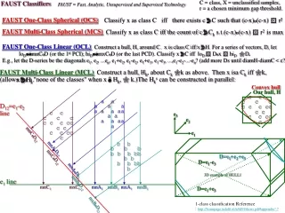
Use a Cut hyperplane between classes. Cut at midpoint between means. PR = P(X dot d)<a vomV vomR d-line d v2 v1 std of these distances from origin along the d-line = std(R) a FAUST Classifier (supervised) a = (mR+(mV-mR)/2)od = (mR+mV)/2o d D≡ mRmV d=D/|D| Training ≡ choosing "cut-hyper-plane" (CHP), which is always an (n-1)-dimensionl hyperplane cutting the space in two. Classify x ≡ If xod<a, classify as R, else V. To classify a set, form the set mask pTree for the set of points and apply We can improve accuracy, e.g., by considering the dispersion within classes when placing the CHP. Use 1. the vector_of_median, vom, to represent each class, rather than mV, vomV ≡ ( median{v1|vV}, median{v2|vV}, ... ) Alternatively, cut using a standard deviation ratio a= std(R)/((std(R)+std(V)) dim 2 r r vv r mR r v v v v r r v mV v r v v r v dim 1