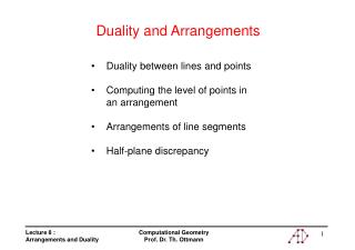
Duality and Arrangements
Duality and Arrangements. Duality between lines and points Computing the level of points in an arrangement Arrangements of line segments Half-plane discrepancy. Different duality mappings. A point p = (a,b) and a line l: y= mx + b are uniquely determined by two parameters.

Duality and Arrangements
E N D
Presentation Transcript
Duality and Arrangements • Duality between lines and points • Computing the level of points in an arrangement • Arrangements of line segments • Half-plane discrepancy
Different duality mappings A point p = (a,b) and a line l: y= mx + b are uniquely determined by two parameters. a) Slope mapping: p * = L(p): y = ax + b b) Polar mapping: p *: ax + by = 1 c) Parabola mapping: p*: y = ax -b d) Duality transform: p = (a,b) is mapped to p *: y = ax – b l: y = mx + b is mapped to l* = (m, -b)
p = (px, py) (px, py) → y = pxx – py, y = mx + b → (m, -b) Characteristics : (p*)* = p = (px, py), (I*)* =l p*: y = pxx – py (p*)* = (px, py) = p (I*)* = I Duality transform
Characteristics of the duality transform 2) Incidence Preserving : p = (px, py) lies onl: y = mx+b iffl* lies on p* p lies on l iff py = mpx + b. l* lies on p* iff (m, -b) fulfills the equation y = pxx – py iff-b = pxm – py.
Characteristics of the duality transform 3) Order Preserving : p lies above l iff l* lies above p* l* = (m,-b) p = (px, py) l: y = mx +b p*: y = pxx - py (px, mpx + b) (m, pxm – py) p lies above lpy > mpx + b l* lies above p*-b > pxm – pyiffpy > pxm + b
Summary Observations: 1. Point p on straight line liff point l * on straight line p * 2. p above l iff l * above p *
Computing the level of points in arrangements Compute for each pair (p,q) of pointsand the straight line l(p,q) defined by p and q: The number of points - above l(p, q) - on l(p, q) - below l(p, q) running time (naive):
Determining the number of points below a line r* l(p,q) q p l(p,q)* r p* q* r is below l(p,q) iff l(p,q)* is below r *
Determining the level of points Define for a setof straight lines for each intersection point p, the number of those straight lines, which run above p. Definition: Level of a point p = # straight lines above p p
Levels of points in an arrangement 0 1 1 2 2 3 2 3 3 3 4
Determining the levels of all Intersections For each straight line: • Compute the level the leftmost intersection with other lines in time O(n) (comparison with all other straight lines). • Walk along the line and update the level at each intersection point 0 1 3 1 pl Run time :O(n²)
Arrangement of a set of n straight lines in the plane Edges Face Vertex
Size of an Arrangement • Theorem : • Let L be a set of n lines in the plane, and let A(L) be the arrangement induced by L. • The number of vertices of A(L) is at most n(n-1)/2. • The number of edges of A(L) is at most n². • 3) The number of faces of A(L) is at most n²/2 + n/2 + 1. • Equality holds in these three statements iff A(L) is simple. Proof : Assume that A(L) is simple. 1) Any pair of lines gives rise to exactly one vertex n(n-1)/2 vertices.2) # of edges lying on a fixed line = 1 + # of intersections on that line with all other lines, which adds up to n. So total number of edges of A(L) = n².
Proof(Contd...) Bounding the # of faces Euler‘s Formula : For any connected planar embedded graph with mv veritces, me edges, mf faces the relation mv – me + mf = 2 holds. We add a vertex vto A(L) to get a connected planar embeddedgraph with v vertices, e arcs and f faces. So we have f = 2 – (v + 1) + e = 2 – (n(n - 1)/2 + 1) + n² = n²/2 + n/2 + 1.
Edges Face Vertex
Storage of an Arrangement Bounding-box R contains all vertices of A(L). R A(L) Store A(L) as doubly connected edge list.
Computation of the Arrangement Modify plane-sweep algorithm for segment intersection: (n² log n), there are max. n² intersections. Incremental algorithm, running in time O(n²) • Compute Bounding box B(L) that contains all vertices of A(L) in its interior. • Construct the doubly connected edge list for the sub- division induced by L on B(L). • for i = 1 to n • do find the edge e on B(L) that contains the leftmost intersection point of li and Ai. • f = the bounded face incident to e. • while f is not the unbounded face • do split f, and set f to be the next intersected face.
Finding the next intersected face g f R Idea: Traverse along the edges of faces intersected by g
Splitting a Face f1 f f2 • a new face • a new vertex • two new half-edges Time : O(1)
Zone Theorem Complexity of the zone of a line: Sum of number of edges and vertices of all intersected faces. Zone Theorem : The complexity of the zone of a line in an arrangement of m lines in the plane is O(m). Proof: By induction on m. (Omitted)
Supersampling Supersampling in Ray Tracing In order to handle arbitrary lines: Choose a random set of points (Supersampling): Shoot many rays through a box, take the average
Computing the Discrepancy Half plane h Unit square U[0,1] x [0,1] S is set of n sample points in U. H = set of all halfplanes Continuous measure of half-plane h H is (h) Discrete measure of h is s(h) s(h):= card (S h) / card(S). The half-plane discrepancy of a set S of n points is the supremum of all differences between the discrete and continuous measures for all halfplanes.
Definition of half-plane discrepancy The discrepancy of h with respect to S, denoted as s (h),is absolute difference between the continuous and discrete measure. s (h) := (h) - s(h). Halfplane discrepancy :
Computing the Discrepancy(contd...) Lemma : Let S be a set of n points in the unit square U. A half-plane h that achieves the maximum discrepancy with respect to S is of one of the following types : 1. h contains one point p S on its boundary. 2. h contains 2 or more points of S on its boundary. The number of type(1) candidates is O(n), and they can be found in O(n) time.
First case: One point px v a 1-py (px, py) a 1 u a 1 A(a) = 1/2 (1 - py+ px tan a) (px + (1 - py) / tan a) Area function has only finitely many extreme values!
Discussion of the area function A(a) = 1/2 (1 - py+ px tan a) (px + (1 - py) / tan a) with tan’ = 1/cos², (1/x)’ = -1/x², chain rule A’(a) = 1/2 (px² / cos² a + (1 - py)²/cos² a tan² a)A’(a) = 0 px² - (1 - py)²/ tan² a tan² a = (1 - py)²/px²