Download
1 / 36
470 likes | 900 Views
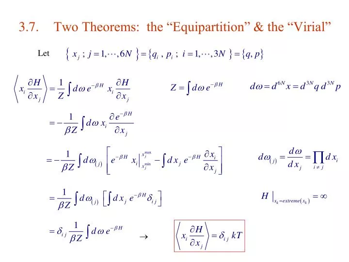
3.7. Two Theorems: the “Equipartition” & the “Virial”. Let. . . Equipartition Theorem. generalized coord. & momenta. Quadratic Hamiltonian :. . . . Fails if DoF frozen due to quantum effects. Equipartition Theorem f = # of quadratic terms in H. Virial Theorem. Virial =.

E N D
3.7. Two Theorems: the “Equipartition” & the “Virial” Let
Equipartition Theorem generalized coord. & momenta Quadratic Hamiltonian : Fails if DoF frozen due to quantum effects Equipartition Theorem f = # of quadratic terms in H.
Virial Theorem Virial = Virial theorem Ideal gas: f comes from collision at walls ( surface S ) : Gaussian theorem : Equipartition theorem : d-D gas with 2-body interaction potential u(r) : Virial equation of state Prob.3.14
3.8. A System of Harmonic Oscillators See § 7.3-4 for applications to photons & phonons. System of N identical oscillators : Oscillators are distinguishable :
Equipartition :
contour closes on the left contour closes on the right as before
Equipartition : fails
Mathematica
g ( E )
Microcanonical Version Consider a set of N oscillators, each with eigenenergies Find the number of distinct ways to distribute an energy E among them. Each oscillator must have at least the zero-point energy disposable energy is R Positive integers • = # of distinct ways to put R indistinguishable quanta (objects) • into N distinguishable oscillators (boxes). • = # of distinct ways to insert N1 partitions into a line of R object.
N = 3, R = 5 Number of Ways to Put R Quanta into N States # of distinct ways to put R indistinguishable quanta (objects) into Ndistinguishableoscillators (boxes). Mathematica
S same as before
Classical Limit Classical limit : equipartition
3.9. The Statistics of Paramagnetism System : N localized, non-interacting, magnetic dipoles in external field H. ( E = 0 set at H = 0 ) (Zrotcancels out ) Dipoles distinguishable
Classical Case (Langevin) Dipoles free to rotate. (c.f. Prob 2.2 ) ( Q , G even in H ) Langevin function Mathematica
CuSO4 K2SO46H2O Magnetization = Strong H, or Low T : Weak H, or High T : Isothermal susceptibility : ( paramagnetic ) Curie’s law C = Curie’s const
Quantum Case J = half integers, or integers = gyromagetic ratio = Lande’s g factor g = 2 for e ( L= 0, S = ½ ) = (signed) Bohr magneton
( M is even in e & // H ) = Brillouin function Mathematica
Limiting Cases Curie’s const =
Dependence on J J ( with g 0 so that is finite ) : x , ~ classical case J= 1/2 ( “most” quantum case ) : g = 2
Gd2(SO4)3 · 8H2O J = 7/2, g = 2 FeNH4(SO4)2 · 12H2O, J = 5/2, g = 2 KCr(SO4)2 J = 3/2, g = 2
3.10. Thermodynamics of Magnetic Systems: Negative T J = ½ , g = 2 M is extensive; H, intensive. Note: everything except M is even in H. U here is the “enthalpy”.
OrderedDisordered (Saturation)(Random) Mathematica
Absolute T • Two equivalent ways to define the absolute temperature scale : • Ideal gas equation. • Efficiency of a Carnot cycle. Dynamically unstable. Violation of the Kelvin & Clausius versions of the 2nd law. U is any thermodynamic potential with S as an independent variable. Definition of the temperature of a system : Impossible if Er is unbounded above.
T < 0 Z finite T 0 if E is unbounded. T < 0 possible if E is bounded. e.g., ( U is even in H ) Usually T > 0 implies U < 0. But T < 0 is also allowable if U > 0. U = 0 set at H = 0
Also
Heat Flow Flow of U (as Q) : High to low. T : 0 0+ : small to large Mathematica
Experimental Realization Let t1= relaxation time of spin-spin interaction. t2= relaxation time of spin-lattice interaction. Consider the case t1<< t2, e.g., LiF with t1= 105 s, t2= 5 min. System is 1st saturated by a strong H ( US = HM < 0 ). H is then reversed. Lattice sub-system has unbounded E spectrum so its T > 0 always. For t1 < t < t2 , spin subsystem in equilibrium; M unchanged US = HM > 0 TS < 0. For t2 < t , spin & lattice are in equilibrium T > 0 & U < 0 for both. T 300K T 350K NMR T ( + ) K
T < 0 requires E bounded above: Usually, K makes E unbounded T < 0 unusual T > 0 requires E bounded below: Uncertainty principle makes E bounded below T > 0 normally
T >> max Let g = # of possible orientations (w.r.t. H ) of each spin
U is larger for smaller • Energy flows from small to large • negative T is hotter than T = +