Download
1 / 69
690 likes | 819 Views
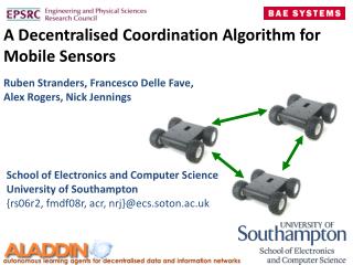
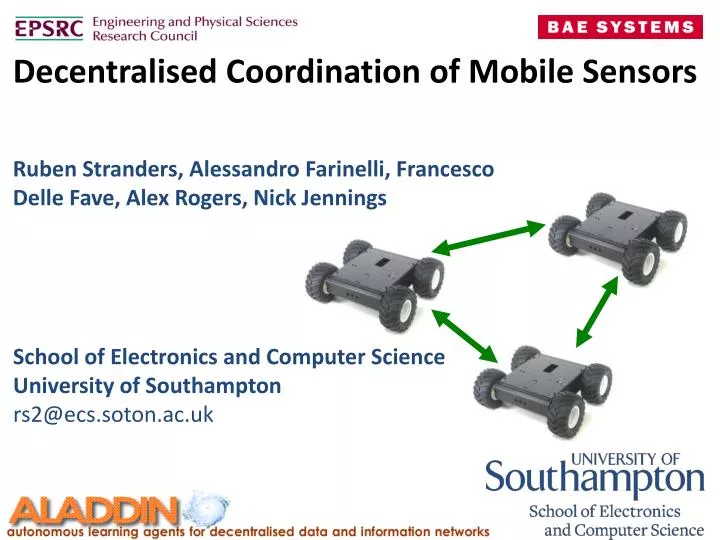
Decentralised Coordination of Mobile Sensors. Ruben Stranders , Alessandro Farinelli , Francesco Delle Fave , Alex Rogers, Nick Jennings. School of Electronics and Computer Science University of Southampton rs2@ecs.soton.ac.uk.

E N D
DecentralisedCoordination of Mobile Sensors Ruben Stranders, Alessandro Farinelli, Francesco DelleFave, Alex Rogers, Nick Jennings School of Electronics and Computer Science University of Southampton rs2@ecs.soton.ac.uk
This presentation focuses on coordinating mobile sensors for information gathering tasks Decentralised Control using Max-Sum Problem Formulation Model Value Coordinate Sensor Architecture
This presentation focuses on coordinating mobile sensors for information gathering tasks Decentralised Control using Max-Sum Problem Formulation Model Value Coordinate Sensor Architecture
Mobile sensor platforms are becoming the de facto means of establishing situational awareness Know what is happening Predict what will happen and understand the impact on the mission “3D” Dull Dirty Dangerous
Currently, there is a strong trend toward making these platforms fully autonomous and cooperative Individual remote controlled vehicles Teams of autonomous vehicles “Auto target engage by 2049…” (My focus was on less nightmarish scenarios….)
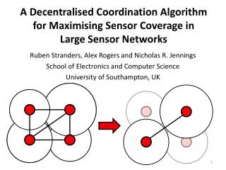
The key challenge is to coordinate a team of sensors to gather information about some features of an environment Sensors • Feature: • moving target • spatial phenomena (e.g. temperature)
We focus on three well known information gathering domains: (1) Pursuit Evasion PE
We focus on three well known information gathering domains: (2) Patrolling P
We focus on three well known information gathering domains: (3) Monitoring Spatial Fields SF
The sensors operate in a constrained environment • No centralised control
The sensors operate in a constrained environment • Limited • Communication
The aim of the sensors is to collectively maximise the value of the observations they take Paths leading to areas already explored - Low value
The aim of the sensors is to collectively maximise the value of the observations they take Paths leading to unexplored areas - High value
The aim of the sensors is to collectively maximise the value of the observations they take PE + P As a result, the target is detected faster
The aim of the sensors is to collectively maximise the value of the observations they take SF As a result, the predictive variance is minimised
This presentation focuses on coordinating mobile sensors for information gathering tasks Decentralised Control using Max-Sum Problem Formulation Model Value Coordinate Sensor Architecture
This presentation focuses on coordinating mobile sensors for information gathering tasks Decentralised Control using Max-Sum Problem Formulation Model Value Coordinate Sensor Architecture
To solve this coordination problem, we had to address three challenges How to modelthe problem? How to value potential samples? How to coordinateto gather samples of highest value?
The three central challenges are clearly reflected in the architecture of our sensing agents Incoming negotiation messages Sensing Agent Samples received from neighbouring agents Value of potential samples Information processing Samples from own sensor Model Value Model of Environment Action Selection Coordinate Move Raw samples Outgoing negotiation messages Samples sent to neighbouring agents
Incoming negotiation messages Sensing Agent Samples received from neighbouring agents Value of potential samples Information processing Samples from own sensor Model of Environment Action Selection Move Raw samples Model Outgoing negotiation messages Samples sent to neighbouring agents
Each sensor builds its own belief map containing all the information gathered about the target PE + P Map of the probability distribution over the target’s position The map is dynamically updated by fusing the new observation gathered
The sensors model the spatial fields using Gaussian Processes SF Spatial Correlations Weak Strong
The sensors model the spatial fields using Gaussian Processes SF Temporal Correlations Weak Strong
Incoming negotiation messages Sensing Agent Samples received from neighbouring agents Value of potential samples Information processing Samples from own sensor Model of Environment Action Selection Move Raw samples Value Outgoing negotiation messages Samples sent to neighbouring agents
Thevalue of a set of observations is equal to the probability of detecting the target PE + P High probability High value: - target might be there Low probability • Low value: • Target is probably somewhere else
The value of a sample is based on how much it reduces uncertainty High entropy Low entropy Lowvalue: - Small uncertainty reduction High value: - Strong uncertainty reduction SF Prediction Confidence Interval Collected Sample
The sensor agents coordinate using the Max-Sum algorithm Incoming negotiation messages Sensing Agent Samples received from neighbouring agents Value of potential samples Information processing Samples from own sensor Model of Environment Action Selection Move Raw samples Coordinate Outgoing negotiation messages Samples sent to neighbouring agents
To decompose the utility function we use the concept of incremental utility value
The key problem is to maximise the social welfare of the team of sensors in a decentralised way Mobile Sensors Social welfare:
The key problem is to maximise the social welfare of the team of sensors in a decentralised way Variable encode paths
Coordinating over all paths is infeasible: it results in a combinatorial explosion for increasing path length Variable encode paths of finite length Thus, we apply receding horizon control
Our solution: we cluster the neighborhood of each sensor Clusters (now each variable represent a path to the Center of each cluster) Most informative is chosen!
This presentation focuses on coordinating mobile sensors for information gathering tasks Decentralised Control using Max-Sum Problem Formulation Model Value Coordinate Sensor Architecture
This presentation focuses on coordinating mobile sensors for information gathering tasks Decentralised Control using Max-Sum Problem Formulation Model Value Coordinate Sensor Architecture
We can now use Max-Sum to solve the social welfare maximisation problem Optimality Complete Algorithms DPOP OptAPO ADOPT Max-Sum Algorithm Iterative Algorithms Best Response (BR) Distributed Stochastic Algorithm (DSA) Fictitious Play (FP) Communication Cost
The input for the Max-Sum algorithm is a graphical representation of the problem: a Factor Graph Variable nodes Function nodes Agent 3 Agent 1 Agent 2
Max-Sum solves the social welfare maximisation problem by local computation and message passing Variable nodes Function nodes Agent 3 Agent 1 Agent 2
Max-Sum solves the social welfare maximisation problem by local computation and message passing From variable i to function j • From function j to variable i
In acyclic factor graphs, the messages converge to the marginal utility functions B A
In acyclic factor graphs, the messages converge to the marginal utility functions B A In such cases, maximising the marginal utility functions is equivalent to maximising the global objective function Max-Sum is optimal on acyclic factor graphs
To use Max-Sum, we encode the mobile sensor coordination problem as a factor graph Sensor 1 Sensor 2 Sensor 3 Sensor 1 Sensor 2 Sensor 3
To use Max-Sum, we encode the mobile sensor coordination problem as a factor graph Sensor 1 Sensor 2 Paths to the most informative positions Sensor 3 Sensor 1 Sensor 2 Sensor 3
To use Max-Sum, we encode the mobile sensor coordination problem as a factor graph Sensor 1 • Local Utility Functions • Measure value of observations along paths Sensor 2 Sensor 3 Sensor 1 Sensor 2 Sensor 3
Unfortunately, the straightforward application of Max-Sum is too computationally expensive From variableito function j From function j to variable i
Unfortunately, the straightforward application of Max-Sum is too computationally expensive From variableito function j From function j to variable i Bottleneck!
Therefore, we developed two general pruning techniques that speed up Max-Sum Goal: Make as small as possible
Therefore, we developed two general pruning techniques that speed up Max-Sum Goal: Make as small as possible Try to prune the action spaces of individual sensors Try to prune joint actions
The first pruning technique prunes individual actions by identifying dominated actions
The first pruning technique prunes individual actions by identifying dominated actions ↑ [1, 2] ↓ [3, 4] 1. Neighbours send bounds ↑ [2, 2] ↓ [1, 1] ↑ [5, 6] ↓ [0, 1]
The first pruning technique prunes individual actions by identifying dominated actions ↑ [1, 2] ↓ [3, 4] 2. Bounds are summed ↑ [2, 2] ↓ [1, 1] ↑ [5, 6] ↓ [0, 1] ↑ [8, 10] • ↓ [4, 7]