Download
1 / 42
420 likes | 553 Views
Advanced Data Analysis for the Physical Sciences. Dr Martin Hendry Dept of Physics and Astronomy University of Glasgow martin@astro.gla.ac.uk. SUPA Advanced Data Analysis Course, Jan 6th – 7th 2009. SUPA Advanced Data Analysis Course, Jan 6th – 7th 2009. Advanced Numerical Methods

E N D
Advanced Data Analysis for the Physical Sciences Dr Martin Hendry Dept of Physics and Astronomy University of Glasgow martin@astro.gla.ac.uk SUPA Advanced Data Analysis Course, Jan 6th – 7th 2009
SUPA Advanced Data Analysis Course, Jan 6th – 7th 2009 • Advanced Numerical Methods • Part 1: Monte Carlo Methods • Part 2: Fourier Methods
SUPA Advanced Data Analysis Course, Jan 6th – 7th 2009 Part 2: Fourier Methods In many diverse fields physical data is collected or analysed as Fourier components. In this section we briefly discuss the mathematics of Fourier series and Fourier transforms. 1. Fourier Series Any ‘well-behaved’ function can be expanded in terms of an infinite sum of sines and cosines. The expansion takes the form: Joseph Fourier (1768-1830)
SUPA Advanced Data Analysis Course, Jan 6th – 7th 2009 The Fourier coefficients are given by the formulae: These formulae follow from the orthogonality properties of sin and cos:
Some examples from Mathworld, approximating functions with a finite number of Fourier series terms
The Fourier series can also be written in complex form: where and recall that “Fourier's Theorem is not only one of the most beautiful results of modern analysis, but it is said to furnish an indispensable instrument in the treatment of nearly every recondite question in modern physics”
SUPA Advanced Data Analysis Course, Jan 6th – 7th 2009 Fourier Transform: Basic Definition The Fourier transform can be thought of simply as extending the idea of a Fourier series from an infinite sum over discrete, integer Fourier modes to an infinite integral over continuous Fourier modes. Consider, for example, a physical process that is varying in the time domain, i.e. it is described by some function of time . Alternatively we can describe the physical process in the frequency domain by defining the Fourier Transform function . It is useful to think of and as two different representations of the same function; the information they convey about the underlying physical process should be equivalent.
SUPA Advanced Data Analysis Course, Jan 6th – 7th 2009 We define the Fourier transform as and the corresponding inverse Fourier transform as If time is measured in seconds then frequency is measured in cycles per second, or Hertz.
SUPA Advanced Data Analysis Course, Jan 6th – 7th 2009 In many physical applications it is common to define the frequency domain behaviour of the function in terms of angular frequency This changes the previous relations accordingly: Thus the symmetry of the previous expressions is broken.
Fourier Transform: Further properties • The FT is a linear operation: • the FT of the sum of two functions is equal to the sum of their FTs • the FT of a constant times a function is equal to the constant times the FT of the function. • If the time domain function is a real function, then its FT is complex. • However, more generally we can consider the case where is also a • complex function – i.e. we can write • may also possess certain symmetries: even function • odd function Imaginary part Real part
SUPA Advanced Data Analysis Course, Jan 6th – 7th 2009 The following properties then hold: Note that in the above table a star (*) denotes the complex conjugate, i.e. if z = x + i y then z* = x − i y See Numerical Recipes, Section 12.0
SUPA Advanced Data Analysis Course, Jan 6th – 7th 2009 For convenience we will denote the FT pair by It is then straightforward to show that “time scaling” “frequency scaling” “time shifting” “frequency scaling”
SUPA Advanced Data Analysis Course, Jan 6th – 7th 2009 Suppose we have two functions and Their convolution is defined as We can prove the Convolution Theorem i.e. the FT of the convolution of the two functions is equal to the product of their individual FTs. Also their correlation, which is also a function of t , is defined as Known as the lag
SUPA Advanced Data Analysis Course, Jan 6th – 7th 2009 We can prove the Correlation Theorem i.e. the FT of the first time domain function, multiplied by the complex conjugate of the FT of the second time domain function, is equal to the FT of their correlation. The correlation of a function with itself is called the auto-correlation In this case The function is known as the power spectral density, or (more loosely) as the power spectrum. Hence, the power spectrum is equal to the Fourier Transform of the auto-correlation function for the time domain function
SUPA Advanced Data Analysis Course, Jan 6th – 7th 2009 The power spectral density The power spectral density is analogous to the pdf we defined in previous sections. In order to know how much power is contained in a given interval of frequency, we need to integrate the power spectral density over that interval. The total power in a signal is the same, regardless of whether we measure it in the time domain or the frequency domain: Parseval’s Theorem
Often we will want to know how much power is contained in a frequency interval without distinguishing between positive and negative values. In this case we define the one-sided power spectral density: And When is a real function With the proper normalisation, the total power (i.e. the integrated area under the relevant curve) is the same regardless of whether we are working with the time domain signal, the power spectral density or the one-sided power spectral density.
From Numerical Recipes, Chapter 12.0 Time domain One-sided PSD Two-sided PSD
Dirac Delta function Examples (1) (2) Imaginary part Real part
(3) Imaginary part = 0 The sinc function occurs frequently in many areas of physics The function has a maximum at and the zeros occur at for positive integer m
(4) 1 1 t f -1/2 0 1/2 0 (5) Real part t Imaginary part
SUPA Advanced Data Analysis Course, Jan 6th – 7th 2009 i.e. the FT of a Gaussian function in the time domain is also a Gaussian in the frequency domain. (6) f t 0 0
Question 15: If the variance of a Gaussian is doubled in the time domain A the variance of its Fourier transform will be doubled in the frequency domain B the variance of its Fourier transform will be halved in the frequency domain C the standard deviation of its Fourier transform will be doubled in the frequency domain D the standard deviation of its Fourier transform will be halved in the frequency domain
Question 15: If the variance of a Gaussian is doubled in the time domain A the variance of its Fourier transform will be doubled in the frequency domain B the variance of its Fourier transform will be halved in the frequency domain C the standard deviation of its Fourier transform will be doubled in the frequency domain D the standard deviation of its Fourier transform will be halved in the frequency domain
SUPA Advanced Data Analysis Course, Jan 6th – 7th 2009 i.e. the FT of a Gaussian function in the time domain is also a Gaussian in the frequency domain. The broader the Gaussian is in the time domain, then the narrower the Gaussian FT in the frequency domain, and vice versa. (6) f t 0 0
where SUPA Advanced Data Analysis Course, Jan 6th – 7th 2009 Discrete Fourier Transforms Although we have discussed FTs so far in the context of a continuous, analytic function, , in many practical situations we must work instead with observational data which are sampled at a discrete set of times. Suppose that we sample in total times at evenly spaced time intervals , i.e. (for even) [ If is non-zero over only a finite interval of time, then we suppose that the sampled points contain this interval. Or if has an infinite range, then we at least suppose that the sampled points cover a sufficient range to be representative of the behaviour of ].
SUPA Advanced Data Analysis Course, Jan 6th – 7th 2009 We therefore approximate the FT as Since we are sampling at discrete timesteps, in view of the symmetry of the FT and inverse FT it makes sense also to compute only at a set of discrete frequencies: (The frequency is known as the Nyquist (critical) frequency and it is a very important value. We discuss its significance later).
SUPA Advanced Data Analysis Course, Jan 6th – 7th 2009 Discrete Fourier Transform of the Then Note that Hence, there are only independent values. Also, note that So we can re-define the Discrete FT as:
SUPA Advanced Data Analysis Course, Jan 6th – 7th 2009 The discrete inverse FT, which recovers the set of from the set of is Parseval’s theorem for discrete FTs takes the form There are also discrete analogues to the convolution and correlation theorems.
Fast Fourier Transforms Consider again the formula for the discrete FT. We can write it as This is a matrix equation: we compute the vector of by multiplying the matrix by the vector of . In general, this requires of order multiplications (and the may be complex numbers). e.g. suppose . Even if a computer can perform (say) 1 billion multiplications per second, it would still require more than 115 days to calculate the FT.
Fortunately, there is a way around this problem. Suppose (as we assumed before) is an even number. Then we can write where So we have turned an FT with points into the weighted sum of two FTs with points. This would reduce our computing time by a factor of two. Odd values of k Even values of k
SUPA Advanced Data Analysis Course, Jan 6th – 7th 2009 Why stop there, however?... If is also even, we can repeat the process and re-write the FTs of length as the weighted sum of two FTs of length . If is a power of two (e.g. 1024, 2048, 1048576 etc) then we can repeat iteratively the process of splitting each longer FT into two FTs half as long. The final step in this iteration consists of computing FTs of length unity: i.e. the FT of each discretely sampled data value is just the data value itself. … …
SUPA Advanced Data Analysis Course, Jan 6th – 7th 2009 This iterative process converts multiplications into operations. So our operations are reduced to about operations. Instead of 100 days of CPU time, we can perform the FT in less than 3 seconds. The Fast Fourier Transform (FFT) has revolutionised our ability to tackle problems in Fourier analysis on a desktop PC which would otherwise be impractical, even on the largest supercomputers. This notation means ‘of the order of’
SUPA Advanced Data Analysis Course, Jan 6th – 7th 2009 Data Acquisition • Earlier we approximated the continuous function and its FT • by a finite set of discretely sampled values. • How good is this approximation? The answer depends on the form of • and . In this short section we will consider: • under what conditions we can reconstruct and exactly from a set of discretely sampled points? • what is the minimum sampling rate (or density, if is a spatially varying function) required to achieve this exact reconstruction? • what is the effect on our reconstructed and if our data acquisition does not achieve this minimum sampling rate?
SUPA Advanced Data Analysis Course, Jan 6th – 7th 2009 The Nyquist – Shannon Sampling Theorem Suppose the function is bandwidth limited. This means that the FT of is non-zero over a finite range of frequencies. i.e. there exists a critical frequency such that The Nyquist – Shannon Sampling Theorem (NSST) is a very important result from information theory. It concerns the representation of by a set of discretely sampled values for all where
SUPA Advanced Data Analysis Course, Jan 6th – 7th 2009 The NSST states that, provided the sampling interval satisfies then we can exactly reconstruct the function from the discrete samples . It can be shown that is also known as the Nyquist frequency and is known as the Nyquist rate. or less
SUPA Advanced Data Analysis Course, Jan 6th – 7th 2009 We can re-write this as So the function is the sum of the sampled values , weighted by the normalised sinc function, scaled so that its zeroes lie at those sampled values. Normalised sinc function sinc(x) (compare with previous section) Note that when then since Sampled values
SUPA Advanced Data Analysis Course, Jan 6th – 7th 2009 The NSST is a very powerful result. We can think of the interpolating sinc functions, centred on each sampled point, as ‘filling in the gaps’ in our data. The remarkable fact is that they do this job perfectly, provided is bandwidth limited. i.e. the discrete sampling incurs no loss of information about and . (Note that formally we do need to sample an infinite number of discretely spaced values, . If we only sample the over a finite time interval, then our interpolated will be approximate). Suppose, for example, that . Then we need only sample twice every period in order to be able to reconstruct the entire function exactly.
SUPA Advanced Data Analysis Course, Jan 6th – 7th 2009 Sampling at (infinitely many of) the red points is sufficient to reconstruct the function for all values of t, with no loss of information.
SUPA Advanced Data Analysis Course, Jan 6th – 7th 2009 Aliasing There is a downside, however. If is not bandwidth limited (or, equivalently, if we don’t sample frequently enough – i.e. if the sampling rate ) then our reconstruction of and is badly affected by aliasing. This means that all of the power spectral density which lies outside the range is spuriously moved inside that range, so that the FT of will be computed incorrectly from the discretely sampled data. Any frequency component outside the range is falsely translated ( aliased ) into that range.
Consider as shown. Suppose is zero outside the range T. This means that extends to . The contribution to the true FT from outside the range gets aliased into this range, appearing as a ‘mirror image’. Thus, at our computed value of is equal to twice the true value. sampled at regular intervals From Numerical Recipes, Chapter 12.1
How do we combat aliasing? • Enforce some chosen e.g. by filtering to remove the • high frequency components . (Also known as anti-aliasing) • Sample at a high enough rate so that - i.e. at • least two samples per cycle of the highest frequency present To check for / eliminate aliasing without pre-filtering: • Given a sampling interval , compute • Check if discrete FT of is approaching zero as • If not, then frequencies outside the range are • probably being folded back into this range. • Try increasing the sampling rate, and repeat…