Download
1 / 85
850 likes | 1.01k Views
Visibility Algorithms. Roger Crawfis CIS 781 This set of slides reference slides used at Ohio State for instruction by Prof. Machiraju and Prof. Han-Wei Shen. Visibility Determination. AKA, hidden surface elimination. Hidden Lines. Hidden Lines Removed. Hidden Surfaces Removed. Topics.

E N D
Visibility Algorithms Roger CrawfisCIS 781 This set of slides reference slides used at Ohio State for instruction by Prof. Machiraju and Prof. Han-Wei Shen.
Visibility Determination • AKA, hidden surface elimination
Topics • Backface Culling • Hidden Object Removal: Painters Algorithm • Z-buffer • Spanning Scanline • Warnock • Atherton-Weiler • List Priority, NNA • BSP Tree • Taxonomy
y clipped line x 1 y 1 near far clipped line x z 0 1 z image plane near far Where Are We ? • Canonical view volume (3D image space) • Clipping done • division by w • z > 0
Back-face Culling • Problems ? • Conservative algorithm • Real job of visibility never solved
Back-face Culling • If a surface’s normal is pointing in the same general direction as our eye, then this is a back face • The test is quite simple: if N * V > 0 then we reject the surface • If test is in eye-space, then if Nz > 0 reject.
Back-face Culling • Only handles faces oriented away from the viewer: • Closed objects • Near clipping plane does not intersect the objects • Gives complete solution for a single convex polyhedron. • Still need to sort, but we have reduced the number of primitives to sort.
Painters Algorithm • Sort objects in depth order • Draw all from Back-to-Front (far-to-near) • Simply overwrite the existing pixels. • Is it so simple?
Point sorting vs Polygon Sorting • What does it mean to sort two line segments? • Zmin? • Zmax? • Slope? • Length? z
3D Cycles • How do we deal with cycles? • How do we deal with intersections? • How do we sort objects that overlap in Z?
Form of the Input Object types: what kind of objects does it handle? • convex vs. non-convex • polygons vs. everything else - smooth curves, non-continuous surfaces, volumetric data
Form of the output Precision: image/object space? • Object Space • Geometry in, geometry out • Independent of image resolution • Followed by scan conversion • Image Space • Geometry in, image out • Visibility only at pixel centers
Object Space Algorithms • Volume testing – Weiler-Atherton, etc. • input: convex polygons + infinite eye pt • output: visible portions of wireframe edges
Image-space algorithms • Traditional Scan Conversion and Z-buffering • Hierarchical Scan Conversion and Z-buffering • input: any plane-sweepable/plane-boundable objects • preprocessing: none • output: a discrete image of the exact visible set
Conservative Visibility Algorithms • Viewport clipping • Back-face culling • Warnock's screen-space subdivision
Z-buffer • Z-buffer is a 2D array that stores a depth value for each pixel. • InitScreen: for i := 0 to N dofor j := 1 to N doScreen[i][j] := BACKGROUND_COLOR; Zbuffer[i][j] := ; • DrawZpixel (x, y, z, color)if (z <= Zbuffer[x][y]) thenScreen[x][y] := color; Zbuffer[x][y] := z;
Z-buffer: Scanline I. foreach polygondoforeach pixel (x,y) in the polygon’s projectiondoz := -(D+A*x+B*y)/C; DrawZpixel(x, y, z, polygon’s color); II. foreach scan-liney doforeach “in range” polygon projectiondo for each pair (x1, x2) of X-intersections dofor x := x1 to x2doz := -(D+A*x+B*y)/C; DrawZpixel(x, y, z, polygon’s color); If we know zx,y at (x,y) then: zx+1,y = zx,y - A/C
Incremental Scanline On a scan line Y = j, a constant Thus depth of pixel at (x1=x+Dx,j) , since Dx = 1,
Incremental Scanline (contd.) • All that was about increment for pixels on each scanline. • How about across scanlines for a given pixel ? • Assumption: next scanline is within polygon , since Dy = 1,
P3 P4 P2 ys za zp zb P1 Non-Planar Polygons Bilinear Interpolation of Depth Values
Non Trivial Example ? Rectangle: P1(10,5,10), P2(10,25,10), P3(25,25,10), P4(25,5,10) Triangle: P5(15,15,15), P6(25,25,5), P7(30,10,5) Frame Buffer: Background 0, Rectangle 1, Triangle 2 Z-buffer: 32x32x4 bit planes
Z-Buffer Advantages • Simple and easy to implement • Amenable to scan-line algorithms • Can easily resolve visibility cycles • Handles intersecting polygons
Z-Buffer Disadvantages • Does not do transparency easily • Aliasing occurs! Since not all depth questions can be resolved • Anti-aliasing solutions non-trivial • Shadows are not easy • Higher order illumination is hard in general
Spanning Scan-Line Can we do better than scan-line Z-buffer ? • Scan-line z-buffer does not exploit • Scan-line coherency across multiple scan-lines • Or span-coherence ! • Depth coherency • How do you deal with this – scan-conversion algorithm and a little more data structure
Spanning Scan Line Algorithm • Use no z-buffer • Each scan line is subdivided into several "spans" • Determine which polygon the current span belongs to • Shade the span using the current polygon’s color • Exploit "span coherence" : • For each span, only one visibility test needs to be done • Assuming no intersecting polygons.
Spanning Scan Line Algorithm • A scan line is subdivided into a sequence of spans • Each span can be "inside" or "outside" polygon areas • "outside“: no pixels need to be drawn (background color) • "inside“: can be inside one or multiple polygons • If a span is inside one polygon, the pixels in the span will be drawn with the color of that polygon • If a span is inside more than one polygon, then we need to compare the z values of those polygons at the scan line edge intersection point to determine the color of the pixel
Determine a span is inside or outside (single polygon) • When a scan line intersects an edge of a polygon • for a 1st time, the span becomes "inside" of the polygon from that intersection point on • for a 2nd time, the span becomes "outside“ of the polygon from that point on • Use a "in/out" flag for each polygon to keep track of the current state • Initially, the in/out flag is set to be "outside" (value = 0 for example). Invert the tag for “inside”.
When there are multiple polygons • Each polygon will have its own in/out flag • There can be more than one polygon having the in/out flags to be "in" at a given instance • We want to keep track of how many polygons the scan line is currently in • If there is more than one polygon "in", we need to perform z value comparison to determine the color of the scan line span
Z value comparison • When the scan line intersects an edge, leaving the top-most polygon, we use the color of the remaining polygon if there is now only 1 polygon "in". • If there is still more than one polygon with an "in" flag, we need to perform z comparison, but only when the scan line leaves a non-obscured polygon.
Many Polygons ! • Use a PT entry for each polygon • When polygon is considered, Flag is true • Multiple polygons can have their flags set to true • Use IPL as active In-Polygon List !
Example Think of ScanPlanes to understand !
Spanning Scan-Line: Example Y AET IPL I x0, ba , bc, xN BG, BG+S, BG II x0, ba , bc, 32, 13, xN BG, BG+S, BG, BG+T, BG III x0, ba , 32, ca, 13, xN BG, BG+S, BG+S+T, BG+T, BG IV x0, ba , ac, 12, 13, xN BG, BG+S, BG, BG+T, BG
Some Facts ! • Scan Line I: Polygon S is in and flag of S=true • ScanLine II: Both S and T are in and flags are disjointly true • Scan Line III: Both S and T are in simultaneously • Scan Line IV: Same as Scan Line II
Spanning Scan-Line build ET, PT -- all polys+BG polyAET := IPL := Nil; for y := yminto ymaxdo e1 := first_item ( AET );IPL := BG;while (e1.x <> MaxX) doe2 := next_item (AET); poly := closest poly in IPL at [(e1.x+e2.x)/2, y] draw_line(e1.x, e2.x, poly-color);update IPL (flags); e1 := e2;end-while;IPL := NIL; update AET;end-for;
Depth Coherence • Depth relationships may not change between polygons from one scan-line to the next scan-line. • These can be kept track using the (active edge table) AET and the (polgon table) PT. • How about penetrating polygons?
Penetrating Polygons Y AET IPL I x0, ba , 23, ad, 13, xN BG, BG+S, S+T, BG+T,BG I’ x0, ba , 23, ec, ad, 13, xN BG, BG+S, BG+S+T, BG+S+T, BG+T, BG False edges and new polygons!
Area Subdivision 1 (Warnock’s Algorithm) Divide and conquer: the relationship of a display area and a polygon after projection is one of the four basic cases:
Warnock : One Polygon if it surrounds then draw_rectangle(poly-color); else begin if it intersects then poly := intersect(poly, rectangle); draw_rectangle(BACKGROUND); draw_poly(poly); end else; What about contained and disjoint ?
Warnock’s Algorithm • Starting with the entire display, we check the following four cases. If none hold, we subdivide the area and repeat, otherwise, we stop and perform the action associated with the case • All polygons are disjoint wrt the area -> draw the background color • Only 1 intersecting or contained polygon -> draw background, and then draw the contained portion of the polygon • There is a single surrounding polygon -> draw the entire area in the polygon’s color • There are more than one intersecting, contained, or surrounding polygons, but there is a front surrounding polygon -> draw the entire area in the polygon’s color • The recursion stops at the pixel level
At A Single Pixel Level • When the recursion stops and none of the four cases hold, we need to perform a depth sort and draw the polygon with the closest Z value • The algorithm is done at the object space level, except scan conversion and clipping are done at the image space level