Download
1 / 109
1.11k likes | 1.17k Views
Learn about control algorithms, linear control methods, feedback systems, and position regulation in robotics with instructor Jacob Rosen at UCLA's MAE 263D course. Explore close-loop control, servo error, stability, position control solutions, and control law partitioning.

E N D
Control of Manipulators Instructor: Jacob Rosen Advanced Robotic - MAE 263D - Department of Mechanical & Aerospace Engineering - UCLA
Introduction – Problem Definition Problem Given: Joint angles (sensor readings) links geometry, mass, inertia, friction, Direct /inverse kinematics & dynamics Compute: Joint torques to achieve an end effector position / trajectory Solution Control Algorithm (PID - Feedback loop, Feed forward dynamic control) Instructor: Jacob Rosen Advanced Robotic - MAE 263D - Department of Mechanical & Aerospace Engineering - UCLA
Introduction – Linear Control • LDF - Linear Control – Valid Method (strictly speaking ) • NLDF - Linear Control – Approximation (practically speaking) • Non Linear Elements (Stiffness, damping, gravity, friction) • Frequently used in industrial practice System Linear Differential Equation System Non Linear Differential Equation Instructor: Jacob Rosen Advanced Robotic - MAE 263D - Department of Mechanical & Aerospace Engineering - UCLA
Feedback & Close Loop Control • Robot (Manipulator) Modeling • Mechanism • Actuator • Sensors (Position / Velocity, Force/toque) • Task (input command) • Position regulation • Trajectory Following • Contact Force control • Hybrid (position & Force ) • Control System – compute torque commands based on • Input • Feedback Instructor: Jacob Rosen Advanced Robotic - MAE 263D - Department of Mechanical & Aerospace Engineering - UCLA
Feedback & Close Loop Control • Open Loop Control System – No feedback from the joint sensor • Impractical - problems • Imperfection of the dynamics model • Inevitable disturbance Instructor: Jacob Rosen Advanced Robotic - MAE 263D - Department of Mechanical & Aerospace Engineering - UCLA
Feedback & Close Loop Control • Close Loop Control System – Use feedback form joint sensors • Servo Error – Difference between the desire joint angle and velocity and the actual joint angle and velocity Instructor: Jacob Rosen Advanced Robotic - MAE 263D - Department of Mechanical & Aerospace Engineering - UCLA
Feedback & Close Loop Control • Control Design • Stability (Servo Errors remain small when executing trajectories) • Close loop performance • Input / Output System • MIMO – Multi-Input Multi-Output • SISO - Single Input Single Output • Current discussion – SISO approach • Industrial Robot – Independent joint control (SISO approach) Instructor: Jacob Rosen Advanced Robotic - MAE 263D - Department of Mechanical & Aerospace Engineering - UCLA
Position Control – Second Order System Position Regulation Instructor: Jacob Rosen Advanced Robotic - MAE 263D - Department of Mechanical & Aerospace Engineering - UCLA
Position Control – Second Order System Position Regulation • Problem • Option 1: The natural response of the mechanical system is under damped and oscillatory • Option 2: The spring is missing and the system never returns to its initial position if disturbed. • Position regulation – maintain the block in a fixed place regardless of the disturbance forces applied on the block • Performance (system response) - critically damped • Equation of motion (free body diagram) Instructor: Jacob Rosen Advanced Robotic - MAE 263D - Department of Mechanical & Aerospace Engineering - UCLA
Position Control – Second Order System Position Regulation • Proposed control law • Close loop dynamics Instructor: Jacob Rosen Advanced Robotic - MAE 263D - Department of Mechanical & Aerospace Engineering - UCLA
Position Control – Second Order System Position Regulation • By setting the control gains ( ) we cause the close loop system to appear to have ANY second order system behaviors that we wish. • For example: Close loop stiffness and critical damping Instructor: Jacob Rosen Advanced Robotic - MAE 263D - Department of Mechanical & Aerospace Engineering - UCLA
Control Law Partitioning • Partition the controller into • Model- Based portion – Make use of the supposed knowledge of . It reduce the system so that it appears to be a unite mass • Servo based portion • Advantages – Simplifying the servo control design – gains are chosen to control a unite mass (i.e. no friction no mass) Servo- Based Model- Based portion Instructor: Jacob Rosen Advanced Robotic - MAE 263D - Department of Mechanical & Aerospace Engineering - UCLA
Control Law Partitioning • Equation of motion • Define the model based portion of the control • Combine • Define • Resulting Instructor: Jacob Rosen Advanced Robotic - MAE 263D - Department of Mechanical & Aerospace Engineering - UCLA
Control Law Partitioning • Control law • Combing the control law with the unit mass ( ) the close loop eq. of motion becomes Servo- Based Model- Based portion Instructor: Jacob Rosen Advanced Robotic - MAE 263D - Department of Mechanical & Aerospace Engineering - UCLA
Control Law Partitioning • Setting the control gains is independent of the system parameters (e.g. for critical damping with a unit mass ) Instructor: Jacob Rosen Advanced Robotic - MAE 263D - Department of Mechanical & Aerospace Engineering - UCLA
Trajectory Following Control • Trajectory Following – Specifying the position of the block as a function of time • Assumption – smooth trajectory i.e. the fist two derivatives exist • The trajectory generation • Define the error between the desired and actual trajectory Instructor: Jacob Rosen Advanced Robotic - MAE 263D - Department of Mechanical & Aerospace Engineering - UCLA
Trajectory Following Control • Servo control • Combined with the eq. of motion of a unite mass leads to • Select to achieve specific performance (i.e. critical damping) • IF • Our model of the system is perfect (knowledge of ) • No noise • Then the block will follow the trajectory exactly (suppress initial error) Instructor: Jacob Rosen Advanced Robotic - MAE 263D - Department of Mechanical & Aerospace Engineering - UCLA
Disturbance Rejection • Control system provides disturbance rejection • Provide good performance in the present of • External disturbance • Noise in the sensors • Close loop analysis - the error equation Instructor: Jacob Rosen Advanced Robotic - MAE 263D - Department of Mechanical & Aerospace Engineering - UCLA
Disturbance Rejection • If is bounded such that • The the solution of the differential equation is also bounded • This result is due to a property of a stable linear system known as bounded-input bounded-output (BIBO) stability Instructor: Jacob Rosen Advanced Robotic - MAE 263D - Department of Mechanical & Aerospace Engineering - UCLA
Disturbance Rejection • Steady state error • The higher the position gain the small will be the steady state error. • In order to eliminate the steady state error a modified control low is used Instructor: Jacob Rosen Advanced Robotic - MAE 263D - Department of Mechanical & Aerospace Engineering - UCLA
Disturbance Rejection • Which results in the error equation • If for then for • Which in a steady state (for constant disturbance) becomes Instructor: Jacob Rosen Advanced Robotic - MAE 263D - Department of Mechanical & Aerospace Engineering - UCLA
Control Problem of Manipulator – Generalized Approach • Equation of Motion (rigid body dynamics) • Inertia matrix n x n • Centrifugal and Coriolis terms n x 1 • Gravity terms n x 1 • Friction Term n x 1 Instructor: Jacob Rosen Advanced Robotic - MAE 263D - Department of Mechanical & Aerospace Engineering - UCLA
Control Problem of Manipulator – Generalized Approach • Partitioning control scheme • Servo control law Instructor: Jacob Rosen Advanced Robotic - MAE 263D - Department of Mechanical & Aerospace Engineering - UCLA
Control Problem of Manipulator – Generalized Approach • The close loop system characterized by the error equation • Note The vector equation is decoupled: the matrix , are diagonal . The equation can be written on a joint by joint basis • Reservations – The ideal performance is unattainable in practice due the many reasons including: • Discrete nature of a digital computer • Inaccuracy of the manipulator model Instructor: Jacob Rosen Advanced Robotic - MAE 263D - Department of Mechanical & Aerospace Engineering - UCLA
Practical Considerations – Time Requirements • Time required to compute the model • Model based control requires to predict joint toques based on the dynamic equation of the manipulator • Digital control / Sampling rate – For every time interval • Read sensor • Calculate feedback command • Send command to the actuator Instructor: Jacob Rosen Advanced Robotic - MAE 263D - Department of Mechanical & Aerospace Engineering - UCLA
Practical Considerations – Time Requirement - Dual Rate Computed Torque • Compute the joint angle based elements of the equation of motion • Lower rate (then the servo) • Pre-compute (look-up table) Solid Line – High rate Servo (e.g 250 Hz) Dashed line – Low rate dynamic model (e.g. 60 HZ) Instructor: Jacob Rosen Advanced Robotic - MAE 263D - Department of Mechanical & Aerospace Engineering - UCLA
Practical Considerations – Lack of Knowledge of the Parameters • The manipulator dynamics is often not known accurately in particular • Friction (parameter & model) • Time dependent dynamics (robot joint wear) • Unknown external load (mass & inertia) – e.g. grasping a tool or a port by the end effector • Summing up all the the disturbance and unknown parameters Instructor: Jacob Rosen Advanced Robotic - MAE 263D - Department of Mechanical & Aerospace Engineering - UCLA
Practical Considerations – Lack of Knowledge of the Parameters • Error equation • Ideal Case • Practical case • Steady state Error • Expressing the disturbance explicitly results in • If the model was exact the right hand side would be zero and so is the error. Instructor: Jacob Rosen Advanced Robotic - MAE 263D - Department of Mechanical & Aerospace Engineering - UCLA
Current Industrial Robot Control SystemsThe Harsh Reality • Most industrial robots nowadays have a PID control scheme • Control law - No use of a model–based component at all • Separate control system for each joint (by a separate micro controller) • No decoupling – the motion of each joint effects the others joints • Error-driven control laws – suppress joint error • Fixed Average gains - approximate critical damping in the middle of the robot workspace (extreme conditions under-damped or over damped) • High gains (as high as possible) – suppress disturbance quickly Instructor: Jacob Rosen Advanced Robotic - MAE 263D - Department of Mechanical & Aerospace Engineering - UCLA
Current Industrial Robot Control SystemsThe Harsh Reality • Gravity terms cause static positioning errors – Gravity compensation (simplest example of model-based controller) • Disadvantage - Gravity terms are coupled. The controller can no longer implemented on a strictly joint-by joint basis. The controller architecture must allow communicating between the joint controllers or must make a use of a central processor rather then individual-joint processors. Instructor: Jacob Rosen Advanced Robotic - MAE 263D - Department of Mechanical & Aerospace Engineering - UCLA
Current Industrial Robot Control SystemsThe Harsh Reality • Approximation of decoupling control (simplifying the dynamic equations) • Ignore and • Include • Simplify by including only for major coupling between axis but not minor cross coupling effects Instructor: Jacob Rosen Advanced Robotic - MAE 263D - Department of Mechanical & Aerospace Engineering - UCLA
Cartesian –Based Control Systems • Joint Based Control • Cartesian based control Instructor: Jacob Rosen Advanced Robotic - MAE 263D - Department of Mechanical & Aerospace Engineering - UCLA
Cartesian –Based Control Systems • Trajectory conversion – difficult in terms of computational expense. The computation that are required are • Simplified computations (in present day systems) Instructor: Jacob Rosen Advanced Robotic - MAE 263D - Department of Mechanical & Aerospace Engineering - UCLA
Cartesian –Based Control Systems • Numerical differentiations • Problem: Amplify noise • Solution 1: When the trajectory is not known • causal filters (past present values) • Solution 2: When the trajectory is known (path preplanned) • Non-causal filters (past present and future values) Instructor: Jacob Rosen Advanced Robotic - MAE 263D - Department of Mechanical & Aerospace Engineering - UCLA
Cartesian –Based Control Systems – Intuitive Schemes Inverse or transpose Jacobian Controller • Inverse Jacobian Controller • Transpose Jacobian Controller Instructor: Jacob Rosen Advanced Robotic - MAE 263D - Department of Mechanical & Aerospace Engineering - UCLA
Cartesian –Based Control Systems – Intuitive Schemes Inverse or transpose Jacobian Controller • The exact dynamic performance of such systems is very complicated • Both scheme can be made stable, but the same performance is not guaranteed over the entire workspace. • We can not choose fixed gains that will result in fixed close loop poles. • The dynamic response of such controllers will vary with arm configuration. Instructor: Jacob Rosen Advanced Robotic - MAE 263D - Department of Mechanical & Aerospace Engineering - UCLA
Cartesian –Based Control Systems – Cartesian decoupling Scheme • Dynamic equations expressed in joint space • Dynamic equations expressed in Cartesian state space (end effector space) Instructor: Jacob Rosen Advanced Robotic - MAE 263D - Department of Mechanical & Aerospace Engineering - UCLA
Cartesian –Based Control Systems – Cartesian decoupling Scheme • Mapping between joint space and cartesian space (end effector) • Multiply both sides by Instructor: Jacob Rosen Advanced Robotic - MAE 263D - Department of Mechanical & Aerospace Engineering - UCLA
Cartesian –Based Control Systems – Cartesian decoupling Scheme Instructor: Jacob Rosen Advanced Robotic - MAE 263D - Department of Mechanical & Aerospace Engineering - UCLA
Cartesian –Based Control Systems – Cartesian decoupling Scheme Solid Line – High rate Servo (e.g 500 Hz) Dashed line – Low rate dynamic model (e.g. 100 HZ) Instructor: Jacob Rosen Advanced Robotic - MAE 263D - Department of Mechanical & Aerospace Engineering - UCLA
Hierarchical Computer Architecture PUMA 560 Instructor: Jacob Rosen Advanced Robotic - MAE 263D - Department of Mechanical & Aerospace Engineering - UCLA
Adaptive Control • The parameters of the manipulator are not known exactly • Mismatch between real and estimated dynamic model parameters leads to servo errors. • Servo errors may be used to adjust the model parameters based on adaptive laws until the errors disappear. • The system learns its own dynamic properties Instructor: Jacob Rosen Advanced Robotic - MAE 263D - Department of Mechanical & Aerospace Engineering - UCLA
Hybrid Control Example 1 Scraping a pint from a surface Control type: Hybrid Control Note: It is possible to control position (velocity) OR force (torque), but not both of them simultaneously along a given DOF. The environment impedance enforces a relashionship between the two Assumption: • The tool is stiff • The position and orientation of the window is NOT known with accurately respect to the robot base. • A contact force normal to the surface transmitted between the end effector and the surface is defined • Position control - tangent to the surface • Force control – normal to the surface Instructor: Jacob Rosen Advanced Robotic - MAE 263D - Department of Mechanical & Aerospace Engineering - UCLA
Hybrid Control of Manipulators Instructor: Jacob Rosen Advanced Robotic - MAE 263D - Department of Mechanical & Aerospace Engineering - UCLA
Introduction – Problem Definition Position control Position control is appropriate when a manipulator is following a trajectory through space Instructor: Jacob Rosen Advanced Robotic - MAE 263D - Department of Mechanical & Aerospace Engineering - UCLA
Introduction – Problem Definition Hybrid Control Fore control or hybrid control (position/force) may be required whenever the end effector comes in contact with the environment Instructor: Jacob Rosen Advanced Robotic - MAE 263D - Department of Mechanical & Aerospace Engineering - UCLA
Introduction – Problem Definition Example 1 Washing a window with a sponge Control type: Position Control Assumption: • The sponge is compliant • The position and orientation of the window is known with respect to the robot base. Instructor: Jacob Rosen Advanced Robotic - MAE 263D - Department of Mechanical & Aerospace Engineering - UCLA
Robotic Systems - Cleaning SKYWASH AEG, Dornier, Fraunhofer Institute, Putzmeister - Germany Using 2 Skywash robots for cleaning a Boeing 747-400 jumbo jet, its grounding time is reduced from 9 to 3.5 hours. The world´s largest cleaning brush travels a distance of approximately 3.8 kilometers and covers a surface of around 2,400 m² which is about 85% of the entire plane´s surface area. The kinematics consist of 5 main joints for the robot´s arm, and an additional one for the turning circle of the rotating washing brush.The Skywash includes database that contains the aircraft-specific geometrical data. A 3-D distance camera accurately positions the mobile robot next to the aircraft. The 3-D camera and the computer determine the aircraft´s ideal positioning, and thus the cleaning process begins. Instructor: Jacob Rosen Advanced Robotic - MAE 263D - Department of Mechanical & Aerospace Engineering - UCLA
Introduction – Problem Definition Example 2 Scraping a pint from a surface Control type: Hybrid Control Note: It is possible to control position (velocity) OR force (torque), but not both of them simultaneously along a given DOF. The environment impedance enforces a relashionship between the two Assumption: • The tool is stiff • The position and orientation of the window is NOT known with accurately respect to the robot base. • A contact force normal to the surface transmitted between the end effector and the surface is defined • Position control - tangent to the surface • Force control – normal to the surface Instructor: Jacob Rosen Advanced Robotic - MAE 263D - Department of Mechanical & Aerospace Engineering - UCLA
Hybrid Control – Strategy • A hybrid control strategy consists of three elements: • Compliance Frame • Selection Matrix • Force and velocity commands • Notes: • Assumption must be made about the environment • A given strategy may work only over a limited range of conditions Instructor: Jacob Rosen Advanced Robotic - MAE 263D - Department of Mechanical & Aerospace Engineering - UCLA