Chapter 7 End-to-End Data

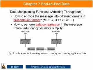
1. Chapter 7 End-to-End Data Outline 7.1 Presentation Formatting 7.2 Data Compression

2. 7.2 Data Compression • Encoding and Compression • Huffman codes • Lossless • data received = data sent • used for executables, text files, numeric data • Lossy • data received does not != data sent • used for images, video, audio

3. 7.2.1 Lossless Compression Algorithms • Run Length Encoding (RLE) • example: AAABBCDDDD encoding as 3A2B1C4D • good for scanned text (8-to-1 compression ratio) • can increase size for data with variation (e.g., some images) • Differential Pulse Code Modulation (DPCM) • example AAABBCDDDD encoding as A0001123333 • change reference symbol if delta becomes too large • works better than RLE for many digital images (1.5-to-1)

4. Dictionary-Based Methods • Build dictionary of common terms • variable length strings • Transmit index into dictionary for each term • Lempel-Ziv (LZ) is the best-known example • Commonly achieve 2-to-1 ration on text • Variation of LZ used to compress GIF images • first reduce 24-bit color to 8-bit color • treat common sequence of pixels as terms in dictionary • not uncommon to achieve 10-to-1 compression (x3)

5. 7.2.2 Image Compression (JPEG) • JPEG: Joint Photographic Expert Group (ISO/ITU) • Lossy still-image compression • Three phase process • process in 8x8 block chunks (macro-block) • grayscale: each pixel is 8 bits (0 white to 255 black) • DCT: transforms signal from spatial domain into and equivalent signal in the frequency domain (loss-less) • apply a quantization to the results (lossy) • RLE-like encoding (loss-less)

6. DCT Phase • DCT is a transformation closely relate to the fast Fourier Transform (FFT) • It takes an 8x8 matrix of pixel values and outputs an 8x8 matrix of frequency coefficients. • DCT breaks this 64-point signal into 64 spatial frequencies. • Imagine yourself moving across a picture in x direction • You would see the value of each pixel varying as some function of x • If this value changes slowly (rapidly) with increasing x, then it as a low (high) spatial frequency. • The low (high) frequencies correspond to the gross (fine) features of the picture. • The idea behind the DCT is to separate the gross features, which is essential to viewing the image, from the fine detail, which is less essential. • DC coefficient – the first coefficient, at location (0,0), the average value of the 64 input pixels. • AC coefficients – The other 63 elements. They add the higher-spatial-frequency information to this average value.

7. Quantization Phase • It’s simply a matter of dropping the insignificant bits of the frequency coefficients. • For example, 45,98,23,66,and 7 with quantum 10 • Then we have 4,9,2,6,and 0 (4 bits vs 7 bits) • Rather than using the same quantum for all 64 coefficients, JPEG uses a quantization table. QuantixedValue(i,j) = IntegerRound(DCT(i,j)/Quantum(i,j)) Where InterRound (x) = x+0.5 if x >=0, x-0.5 if x <0, • When decompression, DCT(i,j) = QuantixedValue(i,j) x Quantum(i,j) • For example, assume DCT(0,0) = 25, then • QuantixedValue(i,j) = 25/3+0.5 = 8 • During decompression, we have 8 x 3 = 24

8. Quantization and Encoding • Quantization Table 3 5 7 9 11 13 15 17 5 7 9 11 13 15 17 19 7 9 11 13 15 17 19 21 9 11 13 15 17 19 21 23 11 13 15 17 19 21 23 25 13 15 17 19 21 23 25 27 15 17 19 21 23 25 27 29 17 19 21 23 25 27 29 31 • Encoding Pattern

9. Encoding Phase • Encodes the quantized frequency coefficients in a compact form. Lossless compression • Zigzag sequence • A form of run length encoding is used to only 0 coefficients, which is significant because many of the later coefficients are 0. • The individual coefficients are then encoded using a Huffman code. • Because the DC coefficient contains a large percentage of the information about the 8x8 block from the source image, and images typically change slowly from block to block, each DC coefficient is encoded as the difference from the previous DC coefficient. (The delta encoding approach).

10. 7.2.3 Video Compression (MPEG) • Motion Picture Expert Group • Lossy compression of video • First approximation: JPEG on each frame • Also remove inter-frame redundancy

11. MPEG (cont) • Frame types • I frames: intrapicture • P frames: predicted picture • B frames: bidirectional predicted picture • Example sequence transmitted as I P B B I B B

12. MPEG (cont) • B and P frames • coordinate for the macroblock in the frame • motion vector relative to previous reference frame (B, P) • motion vector relative to subsequent reference frame (B) • delta for each pixel in the macro block • Effectiveness • typically 90-to-1 • as high as 150-to-1 • 30-to-1 for I frames • P and B frames get another 3 to 5x

13. 7.2.4 Transmitting MPEG • Adapt the encoding • resolution • frame rate • quantization table • GOP (Groups of Pictures) mix • Packetization • Dealing with loss • GOP -induced latency

14. Layered Video • Layered encoding • e.g., wavelet encoded • Receiver Layered Multicast (RLM) • transmit each layer to a different group address • receivers subscribe to the groups they can “afford” • Probe to learn if you can afford next higher group/layer • Smart Packet Dropper (multicast or unicast) • select layers to send/drop based on observed congestion • observe directly or use RTP feedback

15. 7.2.5 Audio Compression (MP3) • CD Quality • 44.1 kHz sampling rate (a sample once every 23 us) • 2 x 44.1 x 1000 x 16 = 1.41 Mbps (16 bits/sample, 2 channels) • 49/16 x 1.41 Mbps = 4.32 Mbps (Synchronization and error correction overhead – 49 bits for each 16 bits sample) • MP3 Compression rates • Layer 1, 384kbps (4), Layer 2, 192kbps (8), Layer 3, 128kbps (12) • Strategy (like MPEG) • split into some number of frequency bands • divide each subband into a sequence of blocks • encode each block using DCT + Quantization + Huffman • trick: how many subbands it elects to use and how many bits assigned to each subband