Download
1 / 20
200 likes | 297 Views
QSH/SHAx states: towards the determination of an helical equilibrium. L. Marrelli acknowledging fruitful discussions with S.Cappello, T.Bolzonella, D.Bonfiglio, A.Boozer, D.F.Escande, M.Gobbin, R.Lorenzini, P.Martin, E.Martines, R.Paccagnella, D. Terranova, R.B.White, M.Zuin. Outline.

E N D
QSH/SHAx states:towards the determination of anhelical equilibrium L. Marrelli acknowledging fruitful discussions with S.Cappello, T.Bolzonella, D.Bonfiglio, A.Boozer, D.F.Escande, M.Gobbin, R.Lorenzini, P.Martin, E.Martines, R.Paccagnella, D. Terranova, R.B.White, M.Zuin
Outline • Present status • QSH/SHAx and helical equilibrium: key experimental evidences • Description of helical (toroidal) equilibrium • Previous work • 2D Helical Grad Shafranov + Ohmic constraint • Work in progress • Numerical and semi-analytical approach: limitations • Using VMEC? • Is the ohmic constraint really necessary for our purposes? • Open issues/Summary
QSH/SHAx vs helical equilibrium • It has been recently proven [1] that in SHAx states the helical pressure correlates with the dominant mode only, despite the residual chaos due to secondary modes • Electron temperature is constant on Single Helicity magnetic surface • Similar evidences are obtained with SXR tomography • Even though we have not measured (yet) the left hand side of the force balance equation… • …this strongly indicates that the SHAx state is an helical equilibrium [1] R.Lorenzini, submitted to Nature Physics
Magnetic field modeling limitations • Magnetic topology is obtained, at present, under the following hypothesis • Zero b axisimmetric (toroidal) equilibrium matching experimental F,Q, assuming a J.B profile of a given parametric radial dependence (J.B=0 at the plasma edge) • Given the axisimmetric profile, helical fields and currents are computed with a zero b perturbative approach (Newcomb equation) matching edge measurements br(a) and bf(a) • In our models, the left hand side of the force balance is zero! • In principle, an axisimmetric pressure can be considered. • What about considering an helical pressure profile? Very difficult.
Equilibrium definition • The force balance equation sets constraints on the shape of the magnetic surfaces • An equilibrium code gives the inverse mapping between physical coordinates (R,Z,f) and the flux coordinates that describe the shape of magnetic surfaces • For diagnostic analysis and for transport codes direct mapping is also required 2D toroidal 2D helical 3D r = flux surface label • = flux coord poloidal angle z= flux coord toroidal angle r = flux surface label h= flux helical angle
Previous work /1 • Helically symmetric equilibria with finite b have been computed [1] assuming • Helical Grad-Shafranov equation: 2D no toroidal effect • Toroidal loop voltage sustains configuration against resistive diffusion: • Ohm’s law constraint: Bz and l=J.B need to be zero on the same surface • Two kind of solutions were found: • Resonant • Non resonant Q=2, F=-0.13 [1] S.Cappello, et al, 26th EPS conference (1999) ECA Vol 23J 981
Previous Work /2 • Numerical determination from Poincaré plots (b=0 assumptions) of helical flux mapping function [1] • aimed at estimating perpendicular transport coefficients inside QSH island [1] M. Gobbin, et al, Phys Plas, (2007) 14, 072305
Previous work /3 • A direct computation of the helical flux function has been recently proposed [1], based on the perturbed toroidal F and poloidal Ψ flux computed with the Newcomb approach Axisymmetric field (toroidal, b=0) Helical angle Single Helicity perturbations [1] E. Martines, Private communication
On going work • While for the toroidal angle we can simply choose… • … how do we compute a “poloidal angle” mapping function? • Is there a “smart” toroidal angle choice that allows an analytical “poloidal angle” dependence? • How can we obtain the inverse mapping functions? • Analytically? • Numerically? • Will this equilibrium be affected by resistive diffusion? • i.e., is the ohmic constraint satisfied? • Probably not
Using VMEC 1 • Can we use a full 3D equilibrium code as the VMEC code instead? • Yes, but with a limitation: it cannot handle toroidal field reversal • Flux surface label is toroidal flux instead of poloidal flux • The Variation Moments Equilibrium Code is routinely used to compute 3D stellarator equilibria, but it is also used for Tokamaks (VMEC/NEMEC) • VMEC minimizes total energy … • … given an appropriate choice of the magnetic field representation in the magnetic flux coordinates (s,q,z) and a spectral representation of the inverse mapping functions • The l function is an important renormalization parameter allowing a compact Fourier representation of R and Z
Using VMEC 2 • Given appropriate boundary constraints an equilibrium can be found. • Fixed boundary: i.e. shape of the Last Closed Magnetic Surface • Pressure profile on s • q profile on s • If necessary, inputs can be adjusted iteratively in order to match additional constraints • Transport codes use VMEC equilibria to compute transport coefficients • Neoclassical transport optimization of stellarators • Ohmic constraint: (See next presentation by A.Boozer) • No matter what code we use for equilibrium reconstruction, using the VMEC data format would allow using stellarator transport codes (See M.Gobbin presentation)
Preparing inputs for VMEC • Pressure profile can be remapped on helical flux surfaces • Work is in progress for the helical (toroidal) q • Different methods are being tested • Direct field line integration • Using cylindrical toroidal and poloidal flux • Does this depend on the assumption on the J.B profile?
Duration of QSH/SHAx states /1 • Even though at present these states’ duration is shorter than the discharge …
Duration of QSH/SHAx states /2 • Even though at present these states’ duration is shorter than the discharge … • … their duration increases with the Lundquist number • The typical resistive diffusion time @1.5MA is about 1-2 s • Given such a difference in time scales, is the ohmic constraint important for describing these states?
Open issues:obtaining the equilibrium • The semi-analytic or numerical approach is based on a zero b or an axisimmetric pressure • Is this accurate enough? No ohmic constraint! • VMEC cannot represent reversed toroidal field • Is this a significant limitation? • Cannot satisfy ohmic constraint with externally applied resonant helicity. • Would the 2D Grad Shafranov approach be sufficient for transport coefficients computation? Probably no: • In 2D, the D coefficient does not depend on the ambipolar field while in 3D it does! [1] • Is pressure a necessary ingredient? • 2D GS + ohmic costraint needed pressure profile • Is it correct to neglect the mean flow? • Post processing of b=0 SpeCyl runs would indicate it is negligible. • Is the ohmic constraint relevant for diagnostic data analysis and transport computations of present day experiments? [1] F.Wagner et al., PPCF 48 (2006) A217
Open issues: using the equilibrium • Once an equilibrium is available: • Diagnostic remapping on helical surfaces; helical power balance • Computation of neoclassical coefficients with stellarator codes • Is neoclassical transport relevant? • In stellarators, the neoclassical ambipolar field is found to affect turbulent transport [1] • Are resistivity and/or viscosity important for equilibrium? • Stability analysis • Are pressure/current driven helical instabilities causing the QSH/SHAx states abrupt termination? • Are we going to learn something about microturbulence? [1] F.Wagner et al., PPCF 48 (2006) A217
Experimental evidences • When the RFX-mod plasma perform a transition to QSH or SHAx [1] states the pressure profile becomes helical • Electron temperature measured by Thomson Scattering, multi-chord double filter • SXR tomography Ensemble averaged electron temperature [2] [1] R.Lorenzini, PRL 2008 [2] F.Bonomo et al, submitted to Phys Plas.
Magnetic topology • The helical shape of the pressure is linked to the topology of the magnetic field lines computed by taking into account all measured MHD modes SHAx QSH But what happens outside the helical region?
Plasma equilibrium and flow • A magnetic configuration is in equilibrium if there is no force acting on the fluid • Usually, the flow velocity v is neglected • Equilibrium codes (VMEC, m&p, etc) solve the equation • According to the boundary conditions and constraints, the degree of complexity of the code increases • E.g. VMEC can compute the shape of flux surfaces (free boundary) • VMEC have also been used to design transport optimized stellarators