Download
1 / 32
320 likes | 486 Views
Precipitation Computed by COSMO-ME model (PR ASS1). Lucio TORRISI Italian Met. Service CNMCA – Pratica di Mare (Rome) l.torrisi@meteoam.it. Overview. PR ASS1 products Description Generation Use Precipitation computed by a NWP model Objective Verification Future developments.

E N D
Precipitation Computed by COSMO-ME model (PR ASS1) Lucio TORRISI Italian Met. Service CNMCA – Pratica di Mare (Rome) l.torrisi@meteoam.it
Overview • PR ASS1 products • Description • Generation • Use • Precipitation computed by a NWP model • Objective Verification • Future developments
PR ASS1 products • The purpose of the computed precipitation products is to support other H-SAF products, e.g. by providing first guess fields or filling occasional gaps in the operational chains for satellite product generation. • PR-ASS1(Quantitative Precipitation Forecast) products are available at fixed times of the day: 00, 03, 06, 09, 12, 15, 18 and 21 UTC. • These products consists of: • accumulated precipitation (AP) over 3, 6, 12 and 24 hours preceding the nominal time; • precipitation rate (PR) at nominal time.
Precipitation rate Maps are in equal latitude/longitude projection. Data in GRIB format
Accumulated precipitation Maps are in equal latitude/longitude projection. Data in GRIB format
PR ASS1 Operational Suite Data assimilation (3DVar) Satellite observations Ground-based and aircraft observations COSMO-ME model integration Precipitation rate Accumulated precipitation End-users and H-SAF central archive The WP-2200 activity is embedded in the development of the operational NWP system of CNMCA.
CNMCA NWP System Data Assimilation 72h • compressible equations • explicit convection 2.8 km • hydrostatic equations • parameterized convection 14 km 24h • compressible equations • parameterized convection 7 km
PR ASS1 Generation PR ASS1 products are generated as forecasts (PR/AP) or forecast differences (AP) from the most appropriate COSMO-ME model run preceding the nominal time (currently two runs a day 00-12 UTC). At 00 UTC: D-1 00 UTC D-1 12 UTC D 00 UTC PR D-1 12 + 12h +12 h D-1 12 + 12h minus D-1 12 + 9h AP 3 +9 h +12 h D-1 12 + 12h minus D-1 12 + 6h AP 6 +6 h +12 h D-1 12 + 12h AP 12 0 h +12 h AP 24 D-1 00 + 24h 0 h +24 h
How to use the GRIB file ftp://hsaf@ftp.meteoam.it/utilities/grib1_decode/ • A decoding programme (C language) for COSMO-ME GRIB files (provide geographical coordinates and values at each grid point) is available in the ftp site as the products, in: • To run the programme: • install grib_api library (http://www.ecmwf.int/products/data/software/download/grib_api.html) • change the GRIB_API_INSTDIR in the Makefile according to your grib api installation directory; • launch make; • use the executable file generated as follows: grib1_decode.ex <grib file>
COSMO-ME Horizontal Grid COSMO-ME uses a rotated lat-lon grid. To derive the geographical coordinates from the rotated ones: where North pole
Precipitation Computed by a NWP Model • Precipitation forecast fields computed by a NWP model will be used in HSAF to provide spatio-temporal continuity to the observed fields, otherwise affected by temporal and spatial gaps due to insufficient and inhomogeneous satellite cover. • “Computed” precipitation by a model is partitioned into two fractions: • the grid-scale precipitation: it refers to the production of precipitation, via atmospheric processes that may be resolved in a NWP model, such as areas where upward motion will ultimately lead to clouds and precipitation (also referred to as explicit condensation) • the parameterized (or convective) precipitation: which is devised to capture the sub-grid scale cumulus convection (by-product of cumulus parameterization schemes) • The partitioning into the components depends on the mesh size
Grid-Scale Clouds/Precipitation Param. • The primary interest in the numerical modelling of grid-scale clouds and precipitation (water-continuity model) is the behaviour of the overall ensemble of particles. • In COSMO model (www.cosmo-model.org) a fully prognostic one-moment bulk water-continuity scheme including five water categories is used (vapour, water, ice, rain, snow, optionally graupel). • The total mass fraction qn of each category is predicted. To accomplish this, the shapes and the size distributions of particles must be assumed and the microphysical processes must be parameterized in terms of qn and the other grid-scale variables where Fqn are the turbulent fluxes (sub-grid scale), Sqn represent cloud microphysical sources and sinks, Pqn denotes the precipitation or sedimentation fluxes
Cumulus Parameterization • A technique used in NWP to predict the collective effects of convective clouds, that may exist within a single grid element, in terms of grid-scale properties • Tiedtke scheme used in COSMO model can be grouped into the family of mass-flux schemes (use simple cloud model to simulate rearrangements of mass in a vertical column) • In the Tiedke scheme a 1-dimensional cloud model is closed by making convection (triggering and intensity) dependent on the moisture supply by large-scale flow convergence and boundary layer turbulence (vertical distribution of heating and drying is estimated using the 1-D cloud model to satisfy the constraints on intensity) • Column equilibrium is supposed for precipitation formed in convective clouds Sqr includes the conversion of cloud water to form rain, the evaporation of rain in the downdraft and below the cloud base
“Tiedke” scheme Cloud top detrainment Updraft entrainment and detrainment Downdraft entrainment and detrainment moisture convergence Adapted from Baldwin (2001)
Objective Verification Objective verification of COSMO-ME precipitation forecasts against SYNOP stations is routinely performed at CNMCA. 6h, 12h and 24h accumulated precipitation scores are calculated for a three month period. MAM (March, April, May) 2007
Contingency Table observed yes no hits false alarms misses correct negatives yes no forecast Objective Verification Precipitation prediction is an example of a yes/no forecast. Some scores (FB, TS, ETS, FAR, etc.) are usually computed from the contingency table. FB=(hits+false alarms)/(hits+misses) The Frequency Bias (FB) measures the ratio of the frequency of forecast events to the frequency of observed events andindicates whether the forecast system has a tendency to underforecast (FB<1) or overforecast (FB>1) events (precipitation frequency). TS=hits/(hits+false alarms+misses) The Threat Score (TS) measures the fraction of observed and/or forecast events that were correctly predicted. The TS is somewhat sensitive to the climatology of the event, tending to give poorer scores for rare events. The Equitable Threat Score is designed to help offset this tendency. ETS=(hits-hits expected by chance)/(hits+false alarms+misses–hits expected by chance) where hits expected by chance = (total forecasts of the event) * (total observations of the event) / (sample size)
Objective Verification 24h Acc. Precipitation - FBI
Objective Verification 24h Acc. Precipitation - ETS
Objective Verification 12h Acc. Precipitation - FBI
Objective Verification 12h Acc. Precipitation - ETS
Objective Verification 06h Acc. Precipitation - FBI
Objective Verification 06h Acc. Precipitation - ETS
Objective Verification Comparison with ECMWF COSMOME vs ECMWF MAM – FBI Acc. Precipitation in 12h
Objective Verification Comparison with ECMWF COSMOME vs ECMWFMAM – ETS Acc. Precipitation in 12h
Objective Verification with a high resolution raingauge network Precipitation verification comparison in 2008/2009 among the several COSMO-Model versions (Elena Oberto, Massimo Milelli - ARPA Piemonte) Presentation at COSMO general meeting 2009 • QPF verification of the 4 model versions at 7 km res. (COSMO-I7, COSMO-7, COSMO-EU, COSMO-ME) with the 2 model versions at 2.8 km res. (COSMO-I2, COSMO-IT) • Specifications: • Dataset: high resolution network of rain gauges coming from COSMO dataset and Civil Protection Department 1300 stations • Method: 24h/6h averaged cumulated precipitation value over 90 meteo-hydrological basins • Model selection: run 00UTC, D+1
Objective Verification From Oberto presentation at COSMO general meeting 2009 Seasonal trend (high thres) • Bias reduction trend, at least during last year • Seasonal cycle: big peak during spring-summertime (convective period) seems to disappear during last summer (… why?) • General good performance during last year • Pronounced underestimation for Cosmo-7 during last seasons
Objective Verification From Oberto presentation at COSMO general meeting 2009 Seasonal trend (high thres) • Slightly improvement trend • Worse performance during summertime (except 2007)
Future Developments • In the CNMCA data assimilation system: • update error statistics in 3DVAR • assimilate new observations (NOAA-19 AMSUA radiances, IASI and GRAS retrievals) • test LETKF (ensemble based) analysis algorithm • use high resolution SST and SWE analysis • In COSMO-ME model: • test Runge-Kutta dynamical core • investigate changes in the cumulus parameterization and microphysics scheme (to reduce the overestimation of small precipitation values during morning and noon and possibly to tune the onset of diurnal convection) • enlarge integration domain and reduce grid spacing
Future developments During CDOP-1 the following improvements are foreseen: • extending the cover to the full H-SAF area. In order not to affect the operational NWP activity at CNMCA, this will probably be implemented by decomposing the area in more frames; • increase the number of runs/day. Currently, although the set of products (integrated over 3, 6, 12 and 24 h and precipitation rate) are disseminated every 3 hours, at synoptic times, they are generated by only two distinct runs/day. It is envisaged to move to 4 runs/day, in order to improve timeliness. • improve the model resolution from the current 7 km to an extent to be assessed for cost/benefit