Download
1 / 27
270 likes | 290 Views
Poznan University of Life Sciences Department of Hydraulic and Sanitary Engineering. METHOD OF LINES (MOL). PDE Geometric Classification P artial D ifferential E qutions The basic idea of the MOL. Hamdi , Schiesser & Griffiths: http://www.scholarpedia.org/article/Method_of_lines.

E N D
Poznan University of Life Sciences Department of Hydraulic and Sanitary Engineering METHOD OF LINES (MOL) • PDE GeometricClassification • PartialDifferentialEqutions • Thebasic idea of the MOL Hamdi, Schiesser & Griffiths: http://www.scholarpedia.org/article/Method_of_lines
PARTIAL DIFFERENTIAL EQUTIONS CHAKTERISTIC AND CLASSIFICATION OF EQUATION • Classification by type • Classification by order SECOND-ORDER PARTIAL DIFFERENTIAL EQUATION • Hyperbolic (równanie hiperboliczne) • Parabolic (równanie paraboliczne) • Elliptic (równanie eliptyczne) PHYSICAL PROBLEMS INVOLVING PDEs • The heat equation Równanie przewodnictwa cieplnego • The wave equation Równanie falowe • The potential equation Równanie Laplace’a RÓWNANIA RÓŻNICZKOWE W HYDRAULICE KORYT OTWARTYCH • Klasyfikacja układu równań różniczkowych I rzędu ELEMENTS OF MOL
ordinary differential equation (równanie różniczkowe zwyczajne) For example: Classification by type
partial differential equation (równanie różniczkowe cząstkowe) For example: Classification by type
second-order ordinary differential equation równanie różniczkowe zwyczajne II rzędu Classification by order • fourth-order partial differential equation • równanie różniczkowe cząstkowe IV rzędu
A quite general second-order partial differential equation of two variables is SECOND-ORDER PARTIAL DIFFERENTIAL EQUATION or • where A, B,C, ... G are constants or are functions of x and y • When G(x,y)=0, the is said to be homogeneous (r. jednorodne); otherwise it is nonhomogeneous (r. nieiejednorodne). • This equation is called quasi-linear because the highest order derivatives appear linearly
The three different classes of second-order quasi-linear equations are given geometric names: Hyperbolic if B2-4AC > 0 (równanie hiperboliczne) Parabolic if B2-4AC = 0 (równanie paraboliczne) Elliptic if B2-4AC < 0 (równanie eliptyczne) SECOND-ORDER PARTIAL DIFFERENTIAL EQUATION
The following linear partial differential equations (1) one-dimensional heat equation (2) one-dimensional wave equation (3) Laplace’s equation play an important role in many areas of physics and engineering. One-dimensional refers to the fact that x denotes dimension, whereas t usually represent time. Równania różniczkowe cząstkowe II rzędu, zwane również równaniami fizyki matematycznej, są stosowane przy rozwiązywaniu problemów w hydromechanice, teorii sprężystości, teorii ciepła, mechanice falowej. PHYSICAL PROBLEMS INVOLVING PARTIAL DIFFERENTIAL EQUATIONS SECOND-ORDER PARTIAL DIFFERENTIAL EQUATION
The heat equationRównanie przewodnictwa cieplnego, r. dyfuzji Because equation has A= 1, B =C= 0 therefore B2-4AC = 0 the equation is parabolic. This equation occurs in the theory of heat flow (that is, heat transferred by conduction) in a rod or thin wire. The function u(x, t) in temperature in the rod.
The heat equationRównanie przewodnictwa cieplnego, r. dyfuzji The constant k is proportional to the thermal conductivity and is called the thermal diffusivity. This equation is sometimes called the diffusion equation since the diffusion of dissolved substances in solution is analogous to the flow of heat in a solid. The function u(x, t) satisfying the partial differential equation in this case represents the concentration of the liquid. Similarly, equation arises in the study of the flow of electricity in the long cable or a transmission line.
The wave equation (Vibrating string)Równanie falowe Because A= 1, B = 0, C = -1/a2therefore B2-4AC >0 the equation is hyperbolic.
The potential equation Równanie Laplace’a • Because A=C= 1, B = 0 therefore B2-4AC >0 the equation is elliptic. Laplace’s equation is encountered in engineering problems in static displacements of membranes, and most often, in problems dealing with potentials such as electrostatic, gravitational, and velocity potentials in fluid mechanics.
Równania różniczkowe w hydraulice koryt otwartych W przypadku kanałów otwartych równania różniczkowe II rzędu spotykamy w dwóch typach zagadnień: • migracja zanieczyszczeń opisana jednowymiarowym równaniem przenoszenia adwekcyjno -dyfuzyjnego. • nieustalony przepływ w kanale opisany uproszczonym modelem w postaci falowej dyfuzyjnej. W obu przypadkach mamy do czynienia z równaniem o ogólnej postaci: gdzie: U – prędkość adwekcji, - stała dyfuzji B2-4AC =0 - 40 = 0, otrzymujemy równanie hiperboliczne
Classification of partial differential equations 2D example http://www.mathematik.uni-dortmund.de/kuzmin/cfdintro/cfd.html
Classification of partial differential equations • PDEs can be classified into hyperbolic, parabolic and elliptic ones • • each class of PDEs models a different kind of physical processes • • the number of initial/boundary conditions depends on the PDE type • • different solution methods are required for PDEs of different type • Hyperbolic equations - Information propagates in certain directions at • finite speeds; the solution is a superposition of multiple simple waves • Parabolic equations - Information travels downstream / forward in time;the solution can be constructed using a marching / time-stepping method • Elliptic equations - Information propagates in all directions at infinite speed; describe equilibrium phenomena (unsteady problems are never elliptic) http://www.mathematik.uni-dortmund.de/kuzmin/cfdintro/cfd.html
Geometric interpretation for a second-order PDE Domain of dependence: x ∈ W which may influence the solution at point P Zone of influence: x ∈ W which are influenced by the solution at point P Hyperbolic PDE Parabolic PDE Elliptic PDE steady supersonic flows unsteady inviscid flows steady boundary layer flows unsteady heat conduction steady subsonic/inviscid incompressible flows http://www.mathematik.uni-dortmund.de/kuzmin/cfdintro/cfd.html
METHOD OF LINES The region is divided into strips by N dividing straightlines (hence the name method of lines) parallel to the y-axis. Since we arediscretising along x, we replace the second derivative with respect to x with itsfinitedifferenceequivalent. y x Sadiku and Obiozor, International Journal of Electrical Engineering Education 37/3
METHOD OF LINES Principle: derivatives in the partial differential equation areapproximatedby linear combinations of function values at the grid points http://www.mathematik.uni-dortmund.de/kuzmin/cfdintro/cfd.html
Approximation of first-order derivatives http://www.mathematik.uni-dortmund.de/kuzmin/cfdintro/cfd.html
One-sided finite difference http://www.mathematik.uni-dortmund.de/kuzmin/cfdintro/cfd.html
Space-time discretization Space discretization: finite differences / finite volumes / finite elements Unknowns: ui(t) time-dependent nodal values / cell mean values Time discretization: (i) before or (ii) after the discretization in space. The space and time variables are essentially decoupled and can be discretizedindependently to obtain a sequence of (nonlinear) algebraic systems http://www.mathematik.uni-dortmund.de/kuzmin/cfdintro/cfd.html
METHOD OF LINES As an example, the equation (10) is generally called the linear advection equation; in physical applications, v is a linear or flow velocity. Although eq. (10) is possibly the simplest PDE, this simplicity is deceptive in thesense that it can be very difficult to integrate numerically since it propagates discontinuities, a distinctive feature of first order hyperbolic PDEs. Hamdi, Schiesser & Griffiths: http://www.scholarpedia.org/article/Method_of_lines
METHOD OF LINES Eq. is termed a conservation law since it expresses conservation of mass, energy or momentum under the conditions for which it is derived, i.e., the assumptions on which theequation is based. Conservation laws are a bedrock of PDE mathematical models in science and engineering, and an extensive literature pertaining to their solution, both analyticaland numerical, has evolved over many years. An example of a first order hyperbolic system (using the notation) is (11) (12) Eqs. (11) and (12) constitute a system of two linear, constant coefficient, first order hyperbolic PDEs. Hamdi, Schiesser & Griffiths: http://www.scholarpedia.org/article/Method_of_lines
Thebasic idea of the MOL The basic idea of the MOL is to replace the spatial (boundary value) derivatives in the PDE with algebraic approximations. Once this is done, the spatial derivatives are no longerstated explicitly in terms of the spatial independent variables. Thus, in effect only the initial value variable, typically time in a physical problem, remains. In other words, with onlyone remaining independent variable, we have a system of ODEs that approximate the original PDE. The challenge, then, is to formulate the approximating system of ODEs. Once thisis done, we can apply any integration algorithm for initial value ODEs to compute an approximate numerical solution to the PDE. Thus, one of the salient features of the MOL is theuse of existing, and generally well established, numerical methods for ODEs. Hamdi, Schiesser & Griffiths: http://www.scholarpedia.org/article/Method_of_lines
Thebasic idea of the MOL To illustrate this procedure, we consider the MOL solution of eq. (10). First we need to replace the spatial derivative with an algebraic approximation. In this case we will use afinite difference (FD) such as where i is an index designating a position along a grid in xandDxis the spacing inx along the grid, assumed constant for the time being. Hamdi, Schiesser & Griffiths: http://www.scholarpedia.org/article/Method_of_lines
Thebasic idea of the MOL Thus, for the left end value ofx, i = 1 and for the right end value ofx, M = 1 i.e., the xgrid in hasM points. Then the MOL approximation of eq. (10) is (19) Note that eq. (19) is written as an ODE since there is now only one independent variable, t. Note also that eq. (19) represents a system of ODEs. Hamdi, Schiesser & Griffiths: http://www.scholarpedia.org/article/Method_of_lines
Thebasic idea of the MOL This transformation of a PDE, eq. (10), to a system of ODEs, eqs. (19), illustrates the essence of the MOL, namely, the replacement of the spatial derivatives, in this case vx so that thesolution of a system of ODEs approximates the solution of the original PDE. Then, to compute the solution of the PDE, we compute a solution to the approximating system of ODEs. But before considering this integration in t, we have to complete the specification of the PDE problem. Since eq. (10) is first order in tand first order inx it requires one IC and oneBC. IC – initial conditions BC – boundary conditions. Hamdi, Schiesser & Griffiths: http://www.scholarpedia.org/article/Method_of_lines