Download
1 / 33
430 likes | 712 Views
Learn about matrices, Gaussian elimination method, systems of linear equations, solutions, elementary row operations, and more in linear algebra. Discover how to solve systems of equations using the Gaussian-Jordan method.

E N D
Linear Algebra 10.1 Gaussian Elimination Method Quiz # 3, Monday 20 on sections: 9.3, 10.1
Objective • Introduction to Matrices • Elementary Row Operations • Gaussian Elimination Method
Matrices • Definition • An equation such as x+3y=9 is called a linear equation.The graph of this equation is a straight line in the x-y plane. • A pair of values of x and y that satisfy the equation is called a solution.
Definition A linear equation in nvariablesx1, x2, x3, …, xn has the form a1 x1 + a2 x2 + a3 x3 + … + anxn = b where the coefficientsa1, a2, a3, …, an and b are real numbers.
Figure 1.3 Many solution) 4x – 2y = 6 6x – 3y = 9 Both equations have the same graph. Any point on the graph is a solution. Many solutions. Figure 1.2 No solution –2x + y = 3 –4x + 2y = 2 Lines are parallel.No point of intersection. No solutions. Solutions for System of Linear Equations Figure 1.1 Unique solution x + 3y = 9 –2x + y = –4 Lines intersect at (3, 2) Unique solution: x = 3, y = 2.
A linear equation in three variables corresponds to a plane in three-dimensional space. • Unique solution( one solution) ※ Systems of three linear equations in three variables:
No solutions • Many solutions
How to solve a system of linear equations? Gaussian Elimination Method. Gaussian –Jordan Method Grammars Rule ….etc
Definition A matrixis a rectangular array of numbers. The numbers in the array are called the elementsof the matrix. • Examples of Matrices
General Form of A Matrix: (i, j)-th entry: Number of rows: m Number of columns: n size: m×n
Size and Type • Location aijrow i, column j location (1,3) = -4 • Identity Matrices • diagonal 1,0,I size
Diagonal matrix: • Square matrix:m = n
Row Echelon Form • Definition • A matrix is in row echelon form if • Any rows consisting entirely of zeros are grouped at the bottom of the matrix. • The first nonzero element of each other row is 1. This element is called a leading 1. • The leading 1 of each row after the first is positioned to the right of the leading 1 of the previous row.
Examples for reduced echelon form () () () () • elementary row operations are used to put a matrix in the row echelon form.
Elementary Transformation Interchange two equations. 2. Multiply both sides of an equation by a nonzero constant. 3. Add a multiple of one equation to another equation. Elementary Row Operation Interchange two rows of a matrix. Multiply the elements of a row by a nonzero constant. Add a multiple of the elements of one row to the corresponding elements of another row. Elementary Row Operations of Matrices
pivot leading 1) pivot pivot Example 2 Use the elementary row operations to find the row echelon form of the following matrix. Solution The matrix is the row echelon form of the given matrix.
Solving Linear Systems by Gaussian Elimination Method • System of linear equations form augmented matrix put the augmented matrix in row echelon from solve by back substitution
= = = x A b Matrix form of a system of linear equations:
row equivalent Solution Analogous Matrix Method Augmented matrix: Equation Method Initial system: Eq2+(–2)Eq1 R2+(–2)R1 Eq3+(–1)Eq1 R3+(–1)R1 Example 3 Solving the following system of linear equation.
Eq3+(2)Eq2 R3+(2)R2 (–1/5)R3 (–1/5)Eq3 Back substitution The solution is The solution is
Example 4 Solving the following system of linear equation. Solution
Example 5 Solve the system Solution
Example 6 Solve, if possible, the system of equations Solution The general solution to the system is
Example 7 Solve the system of equations many sol. Solution
Example 8 Solve the system of equations Solution
0x1+0x2+0x3=1 Example 9 This example illustrates a system that has no solution. Let us try to solve the system Solution The system has no solution.
Example: The system has other nontrivial solutions. Theorem A system of homogeneous linear equations that has more variables than equations has many solutions. Homogeneous System of linear Equations Note. trivial solution
Summary If , then the system is independent If , then the system is dependent If , then the system is inconsistent
Exercises • Ex 55: Find all values of a for which the following system has a unique solution
Ex :Find the interpolating polynomial that passes through the points ( -3,28), (-1,6) and (2,3)