Download
1 / 23
230 likes | 355 Views
Mining for Low Abundance Transcripts in Microarray Data. Yi Lin 1 , Samuel T. Nadler 2 , Hong Lan 2 , Alan D. Attie 2 , Brian S. Yandell 1,3 1 Statistics, 2 Biochemistry, 3 Horticulture, University of Wisconsin-Madison. Key Issues. differential gene expression using mRNA chips

E N D
Mining for Low Abundance Transcripts in Microarray Data Yi Lin1, Samuel T. Nadler2, Hong Lan2, Alan D. Attie2, Brian S. Yandell1,3 1Statistics, 2Biochemistry, 3Horticulture, University of Wisconsin-Madison www.stat.wisc.edu/~yandell/statgen
Key Issues • differential gene expression using mRNA chips • diabetes and obesity study (biochemistry) • lean vs. obese mice: how do they differ? • what is the role of genetic background? • detecting genes at low expression levels • inference issues • formal evaluation of each gene with(out) replication • smoothly combine information across genes • significance level and multiple comparisons • general pattern recognition: tradeoffs of false +/– • modelling differential expression • gene-specific vs. dependence on abundance • R software module www.stat.wisc.edu/~yandell/statgen
Diabetes & Obesity Study • 13,000+ mRNA fragments (11,000+ genes) • oligonuleotides, Affymetrix gene chips • mean(PM) - mean(NM) adjusted expression levels • six conditions in 2x3 factorial • lean vs. obese • B6, F1, BTBR mouse genotype • adipose tissue • influence whole-body fuel partitioning • might be aberrant in obese and/or diabetic subjects • Nadler et al. (2000) PNAS www.stat.wisc.edu/~yandell/statgen
Low Abundance Genes for Obesity www.stat.wisc.edu/~yandell/statgen
Low Abundance Obesity Genes • low mean expression on at least 1 of 6 conditions • negative adjusted values • ignored by clustering routines • transcription factors • I-kB modulates transcription - inflammatory processes • RXR nuclear hormone receptor - forms heterodimers with several nuclear hormone receptors • regulation proteins • protein kinase A • glycogen synthase kinase-3 • roughly 100 genes • 90 new since Nadler (2000) PNAS www.stat.wisc.edu/~yandell/statgen
Obesity Genotype Main Effects www.stat.wisc.edu/~yandell/statgen
Low Abundance on Microarrays • background adjustment • remove local “geography” • comparing within and between chips • negative values after adjustment • low abundance genes • virtually absent in one condition • could be important: transcription factors, receptors • large measurement variability • early technology (bleeding edge) • prevalence across genes on a chip • up to 25% per chip (reduced to 3-5% with www.dChip.org) • 10-50% across multiple conditions • low abundance signal may be very noisy • 50% false positive rate even after adjusting for variance • may still be worth pursuing: high risk, high research return www.stat.wisc.edu/~yandell/statgen
Why not use log transform? • log is natural choice • tremendous scale range (100-1000 fold common) • intuitive appeal, e.g. concentrations of chemicals (pH) • looks pretty good in practice (roughly normal) • easy to test if no difference across conditions • but adjusted values = PM – MM may be negative • approximate transform to normal • very close to log if that is appropriate • handles negative background-adjusted values • approximate -1(F()) by -1(Fn()) www.stat.wisc.edu/~yandell/statgen
Normal Scores Procedure adjusted expression = PM – MM rank order R = rank() / (n+1) normal scores X = qnorm( R ) X = -1(Fn()) average intensity A = (X1+X2)/2 difference D = X1 – X2 variance Var(D | A) 2(A) standardization S = [D –(A)]/(A) www.stat.wisc.edu/~yandell/statgen
7. standardize S=D –center spread 0. acquire data PM,MM 1. adjust for background =PM – MM 2. rank order genes R=rank()/(n+1) 4. contrast conditions D=X1 –X2 A=mean(X) 3. normal scores X=qnorm(R) 5. mean intensity A=mean(X) www.stat.wisc.edu/~yandell/statgen
Robust Center & Spread • center and spread vary with mean expression X • partitioned into many (about 400) slices • genes sorted based on X • containing roughly the same number of genes • slices summarized by median and MAD • median = center of data • MAD = median absolute deviation • robust to outliers (e.g. changing genes) • smooth median & MAD over slices www.stat.wisc.edu/~yandell/statgen
Robust Spread Details • MAD ~ same distribution across A up to scale • MADi = i Si, Si ~ S, i = 1,…,400 • log(MADi ) = log(i) + log(Si), I = 1,…,400 • regress log(MADi) on Ai with smoothing splines • smoothing parameter tuned automatically • generalized cross validation (Wahba 1990) • globally rescale anti-log of smooth curve • Var(D|A) 2(A) • can force 2(A) to be decreasing www.stat.wisc.edu/~yandell/statgen
Anova Model • transform to normal: X = -1(Fn()) • Xijk = + Ci + Gj + (CG)ij + Ejjk • i=1,…,I conditions; j=1,…,J genes; k=1,…,K replicates • Ci = 0 if arrays normalized separately • Zi = 1(0) if (no) differential expression • Variance (Aj =jkXijk /IK) • Var(Xijk | Aj) = (Aj)2+ (Aj)2+ (Aj)2 if Zi = 1 • Var(Xijk | Aj) = (Aj)2+ (Aj)2 if Zi = 0 www.stat.wisc.edu/~yandell/statgen
Differential Expression • Djk = wi Xijk with wi = 0, wi2= 1 • Djk = wi (CG)ij + wi Ejjk • Variance depending on abundance • Var(Djk | Aj) = (Aj)2+ (Aj)2 if Zi = 1 • Var(Djk | Aj) = (Aj)2 if Zi = 0 • Variance depending on gene j ? • Var(Djk | j, Aj) = (Aj)2Vj, with Vj, ~ -1(,) • gene-specific variance • gene function-specific variance www.stat.wisc.edu/~yandell/statgen
gene-specific variance? www.stat.wisc.edu/~yandell/statgen
Bonferroni-corrected p-values • standardized differences • Sj= [Dj–(Aj)]/(Aj) ~ Normal(0,1) ? • genes with differential expression more dispersed • Zidak version of Bonferroni correction • p = 1 – (1 – p1)n • 13,000 genes with an overall level p = 0.05 • each gene should be tested at level 1.95*10-6 • differential expression if S > 4.62 • differential expression if |Dj–(Aj)| > 4.62(Aj) • too conservative? weight by Aj? • Dudoit et al. (2000) www.stat.wisc.edu/~yandell/statgen
comparison of multiple comparisons uniform j/(1+n)grey p-value black nominal .05 red Holms purple Sidak blue Bonferroni www.stat.wisc.edu/~yandell/statgen
Patterns of Differential Expresssion • (no) differential expression: Z = (0)1 • Sj|Zj ~ density fZ • f0 = standard normal • f1 = wider spread, possibly bimodal • Sj ~ density f = (1 – 1)f0 +(1 – 1)f1 • chance of differential expression: 1 • prob(Zj = 1) = 1 • prob(Zj = 1 | Sj ) = 1 f1(Zj) / f(Zj) www.stat.wisc.edu/~yandell/statgen
density of standardized differences • S =[D –(A)]/(A) • f = black line • standard normal • f0 = blue dash • differential expression • f1 = purple dash • Bonferroni cutoff • vertical red dot www.stat.wisc.edu/~yandell/statgen
Looking for Expression Patterns • differential expression: D = X1 – X2 • S = [D –center]/spread ~ Normal(0,1) ? • classify genes in one of two groups: • no differential expression (most genes) • differential expression more dispersed than N(0,1) • formal test of outlier? • multiple comparisons issues • posterior probability in differential group? • Bayesian or classical approach • general pattern recognition • clustering / discrimination • linear discriminants (Fisher) vs. fancier methods www.stat.wisc.edu/~yandell/statgen
Related Literature • comparing two conditions • log normal: var=c(mean)2 • ratio-based (Chen et al. 1997) • error model (Roberts et al. 2000; Hughes et al. 2000) • empirical Bayes (Efron et al. 2002; Lönnstedt Speed 2001) • gene-specific Dj ~ , var(Dj) ~-1, Zj ~ Bin(p) • gamma • Bayes (Newton et al. 2001, Tsodikov et al. 2000) • gene-specific Xj ~, Zj ~ Bin(p) • anova (Kerr et al. 2000, Dudoit et al. 2000) • log normal: var=c(mean)2 • handles multiple conditions in anova model • SAS implementation (Wolfinger et al. 2001) www.stat.wisc.edu/~yandell/statgen
R Software Implementation • quality of scientific collaboration • hands on experience of researcher • save time of stats consultant • raise level of discussion • focus on graphical information content • needs of implementation • quick and visual • easy to use (GUI=Graphical User Interface) • defensible to other scientists • public domain or affordable? • www.r-project.org www.stat.wisc.edu/~yandell/statgen
library(pickgene) ### R library library(pickgene) ### create differential expression plot(s) result <- pickgene( data, geneID = probes, renorm = sqrt(2), rankbased = T ) ### print results for significant genes print( result$pick[[1]] ) ### density plot of standardized differences pickedhist( result, p1 = .05, bw = NULL ) www.stat.wisc.edu/~yandell/statgen