Monopoly
Chapter 12. Monopoly. Market structure or environment in which one firm produces a good or service with no close substitutes. 12- 1. Chapter Outline. Defining Monopoly Five Sources Of Monopoly The Profit-maximizing Monopolist A Monopolist Has No Supply Curve Adjustments In The Long Run

Monopoly
E N D
Presentation Transcript
Chapter 12 Monopoly Market structure or environment in which one firm produces a good or service with no close substitutes. 12-1
Chapter Outline • Defining Monopoly • Five Sources Of Monopoly • The Profit-maximizing Monopolist • A Monopolist Has No Supply Curve • Adjustments In The Long Run • Price Discrimination • The Efficiency Loss From Monopoly • Public Policy Toward Natural Monopoly 12-2
What is a Monopoly? Monopoly:a market structure in which a single seller of a product with no close substitutes serves the entire market. • A monopoly has significant control over the price it charges (Contrast: In Chap. 11, a typical firm is price-taker in P X Q while in Chap. 12, the firm is a price-maker, i.e. adjusts P to influence Q). Five Sources Of Monopoly • Exclusive Control over Important Inputs • Economies of Scale –major source of monopoly of the 5! • Patents • Network Economies, e.g. Microsoft’s Window operating system . Often driven by the demand side and not the Supply side!“Network externalities” means that there are benefits if many people use the same thing. • Government Licenses or Franchises, e.g. college campuses granting exclusive rights to either Coke or Pepsi 12-3
Figure 12.1: Natural Monopoly • When there is only 1 firm, the LAC is LACQ* for producing Q*. • With 2 firms, the LAC is LACQ*/2 for Q*/2 • Thus, when the LAC is declining (due to economies of scale/size), it is optimal to have a single producer. • For allowing such a monopoly, the government often regulates its behavior, e.g. SMUD in Sacramento. 12-4
The Profit-maximizing Monopolist The monopolist’s goal is to maximize economic profit. • In the short run this means to choose the level of output for which the difference between total revenue and short-run total cost is greatest. Revenue for the Monopolist • As price falls, total revenue for the monopolist does not rise linearly with output. • Instead, it reaches a maximum value at the quantity corresponding to the midpoint of the demand curve (ϵp=1)after which it again begins to fall. • Total revenue (TR) reaches its maximum value when the price elasticity of demand is unity (εP=1) 12-5
P= 80 – (1/5)*Q TR= 80Q – (1/5)Q2 MR =dTR/dQ= 80 – 2/5Q MR εP = 1 when TR is maximum Figure 12.2: The Total Revenue Curve for a Perfect Competitor Figure 12.3: Demand, Total Revenue, and Elasticity The MR curve is identical to the AR, P and the demand curve facing a typical firm. Thus, P=MR=AR in Chap.11. The slope of the MR is twice the slope of the D=AR curve. That is, the MR curve lies below the D=AR curve in Chap. 12. 12-6
Figure 12.4: Total Cost, Revenue,and Profit Curves for a Monopolist Demand: P = 100 -2Q Max profit Econ Profit is positive • The Profit-maximizing Monopolist • Optimality condition for a monopolist:a monopolist maximizes profit by choosing the level of output where marginal revenue equals marginal cost (MR=MC is still in Monopoly as it was in Perfect Competition). 12-7
XXX = LOSS ZZZ = GAIN ∆ TR = ∆PQ + P∆Q + ∆P∆Q 0 Figure 12.6: Marginal Revenueand Position on the Demand Curve Figure 12.5: Changes in Total Revenue Resulting from a Price Cut • If Q0 is left of M, GAIN > LOSS • If Q1 is right of M, GAIN<LOSS • If Q is at M, then GAIN = LOSS Area B = P ∆Q = 50x50 =$2500= GAIN Area A = ∆PQ = (60 – 50) x100 =$1000 = LOSS 12-8
Figure 12.7: The Demand Curve and Corresponding Marginal Revenue Curve εP = (∆Q/∆P)*(P/Q) MRQ = P(1 – 1/| εP |) • Marginal Revenue And Elasticity • The less elastic demand is with respect to price, the more price will exceed marginal revenue. • For all elasticity values less than 1 in absolute value marginal revenue will be negative (εP <1and MR<0) • For all elasticity values larger than 1 in absolute value marginal revenue will be positive ((εP >1and MR>0) • For all elasticity values equal to1 in absolute value marginal revenue will be zero ((εP =1and MR=0) 12-9
Figure 12.8: A Specific Linear Demand Curve and the Corresponding Marginal Revenue Curve Since Q = 4 –(1/3)P (write it in terms of P) implies that P = 12 -3Q, then TR= PQ =TR = (12 – 3Q)*Q = 12Q – 3Q2 Then the slope of the TR = MR = dTR/dQ = 12 - 6Q OR that the slope of the TR curve is twice the slope of demand curve! 12-10
Figure 12.9: The Profit-Maximizing Price and Quantity for a Monopolist Ch11: (1)P =MR & (2)MR=MC and thus (3) P=MC at equilibrium Ch 12: (1)P > MR & (2) MR = MC and hence (3) P>MC at equilibrium 12-11
Figure 12.10: The Profit-Maximizing Price and Quantity for Specific Cost and Demand Functions Given P = 100 -2Q; STC = 640 + 20Q, MC=20, find optimal output, price and profits. Set MR = MC 100 – 4Q = 20 or Q= 20; P = 100 – 2* 20 = 60. The profit = 60*20 –(640 + 20*20) =$160 OR (P – ATC)Q = (60 – 52)*20 12-12
The Profit-maximizing Monopolist • If a monopolist’s goal is to maximize profits, she will never produce an output level on the inelastic portion of her demand curve. • The profit-maximizing level of output must lie on the elastic portion of the demand curve. Monopolist’s Profit-Maximizing Mark-up Combine MR= P(1 – 1/|εP |) and MR =MC to yield, (P-MC)/P = 1/|εP |= mark-up over MC • If εP =∞, then the mark-up is zero • If εP =0, then the mark-up has no limit Example: Suppose εP = 2 => a mark-up =1/2 =50% 12-13
Figure 12.11: A Monopolist who Should Shut Down in the Short-Run At MC =MR (Point A), P < AVC, this implies thatP < ATC. Thus, the monopolist must shutdown A • The Profit-maximizing Monopolist • Shutdown condition for a monopolist:he should cease production whenever average revenue (AR ≈D =price value on the demand curve) is less than average variable cost at every level of output. 12-14
A Monopolist Has No Supply Curve • The monopolist is a price maker. • When demand shifts rightward, elasticity at a given price may either increase or decrease, and vice-versa. • So there can be no unique correspondence between the price (P) a monopolist charges and the amount she/he chooses to produce. • Monopoly has a supply rule, which is to equate marginal revenue and marginal cost (MR=MC) Example: • P = 100 -2Q so Q=50(if P=0); TC = 640 + 20Q; MC=20 and Q*=20 and P*=60 Versus • P = 100 - Q so Q=100 (if P=0); TC = 640 + 20Q;MC=20 and Q*=40 and P*=60 Identical MCs, different demand curves give rise to different optimal output values 12-15
Figure 12.12: Long-Run Equilibriumfor a Profit-Maximizing Monopolist We assume a given technology. Choose Q* where LMC =MR (point A) and choose capital stock (K) in the SR that gives rise to SMC* and ATC* K A 12-16
Figure 12.13: The Profit-Maximizing Monopolist Who Sells in Two Markets Given MR1 = MR2 MC = MR* = (MR1 +MR2) • Price Discrimination • Price discrimination:a practicewhere the monopolist charge different prices to different buyers, i.e. converting CS from buyers to itself! • Third-degree price discrimination:charging different prices to buyers in completely separate markets. • First-degree price discrimination:is the term used to describe the largest possible extent of market segmentation. 12-17
MC =Q; Home demand (H) P=30-Q, Foreign (F)=12; MRH =30 – 2Q Charge the maximum the buyer is willing to pay Figure 12.14: A Monopolist witha Perfectly Elastic Foreign Market Figure 12.15: Perfect Price Discrimination Total: MRF =12, MC =Q; Q=12 Domestic : MRH =MRF => 30-2QH=12 so QH =9 Foreign MRF =12 => 12-9 =3=QF 12-18
For this monopolist, set MR =MC implies that the D curve is the MR! Creams off all CS! Seller posts different prices, with declines as volume purchased increases CS captured by the monopolist Figure 12.16: The Perfectly Discriminating Monopolist Figure 12.17: Second-Degree Price Discrimination Second-Degree Price Discrimination Second-degree price discrimination:price discrimination where the same rate structure is available to every consumer and the limited number of rate categories tends to limit the amount of consumer surplus that can be captured. 12-19
Figure 12.18: A Perfect Hurdle • Idea: seller induces buyers with high elastic demand to identify themselves. That is, the seller sets up a hurdle of some sort that buyers have to hop over. • Example: hurdle could be a discount coupon (buy it now for retail and get a coupon; wait for 6 -8 weeks to get a rebate) • Fig. 12.18 shows a perfect hurdle – PH is a regular and PL is the discount price. Without a hurdle, QL would have been excluded from the market! • Another example: multiple prices on any aircraft! 12-20
Figure 12.19: The Welfare Loss froma Single-Price Monopoly Perfect Comp (Chap. 11) – largest total surplus – all potential trades completed; in Monopoly, this requires production QC at price PC. However, the optimals here are Q* < QC and P*>PC. Still exists some trades that could be completed. The loss to society Loss to Consumers • The Efficiency Loss From Monopoly • Deadweight loss from monopoly:the loss of efficiency due to the presence of a Monopoly. • --Is the result of failure to price discriminate perfectly. 12-21
Public Policy Toward Natural Monopoly • State Ownership And Management • State Regulation Of Private Monopolies • Exclusive Contracting For Natural Monopoly • Vigorous Enforcement Of Antitrust Laws • A Laissez-faire Policy Toward Natural Monopoly 12-22
Figure 12.20: A Natural Monopoly • Suppose TC = F + MQ where Q = output and M = MC: Ideally, produce Q** and sell at M. Problem: Production at Q* implies loss since P= M< ATC • In reality, the monopolist produces Q* and sells at P*. This reality earns the monopolist (1) profits = π (Fairness Objection) and (2) causes loss of CS =Area S (Efficiency objection – P > MC and results in a loss of CS). • These objections lead to 5 ways to remedy the problem. 12-23
Figure 12.21: Cross-Subsidizationto Boost Total Output under State Regulation of Private Firms • If not state ownership, then state regulation. But that has the problem of having rate-of-return distortions, if the monopolist serves more than one separate market. • In the Figure, the ATC include the (a) allowed rate of profit and (b) the rate of profit exceeds the cost of capital. Monopolist is allowed rate of return which exceeds the cost of capital, the incentive is to set P way above MC in the inelastic market (Panel A) and earn π1>0 and use these profits to subsidize Market 2 where P<ATC, i.e. π2<0 . This cross-subsidization, unless disallowed, can enable a monopolist to retain significant power in the inelastic market! 12-24
Figure 12.22: The Efficiency Losses from Single-Price and Two-Price Monopoly • Idea: Do nothing, i.e. let the free market rule. Two objections: (a) fairness and (b) efficiency problems. • Without the Hurdle Model, the inefficiency remains since there is only one single price (Panel A) where the loss of CS to society = CS. • Assume that TC = F + MQ • With the Hurdle model, the monopolist charges different prices to buyers who manage the hurdle on the elastic portion of the demand curve. In the limit, he charges P = MC. The efficiency loss in terms of CS is only Z<W. 12-25
Figure 12.23: Does MonopolySuppress Innovation? • Common Assertion: Monopolists deprive consumers of beneficial technological innovations., i.e. there are social costs to monopoly. • Monopolist currently can produce bulbs that last 1,000 hours at $1.00/per bulb hour. Finds that he can produce bulb that lasts 10,000 hours at the same cost (thus, the cost per bulb hr is $0.10). The demand curve is D and the marginal revenue is MR. • Profit when ATC = $1.00 is area ABCE but when ATC = $0.10, profit is area FGHK. • The monopolist will produce new bulbs since Area FGHK > Area ABCE. Thus, the assertion may not always be true! 12-26