Download
1 / 7

E N D
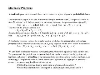
Stochastic ProcessesA stochastic process is a model that evolves in time or space subject to probabilistic laws.The simplest example is the one-dimensional simple random walk.. The process starts in state X0 at time t = 0. Independently, at each time instance, the process takes a jump Zn: Prob { Zn = -1} = q, Prob { Zn = +1} = p and Prob { Zn = 0 } = 1 - p - q.The state of the process at time n is Xn = X0 + Z1 + Z2 + … + Zn.Assume for convenience that X0 = 0. Since E[ Zn] = p - q and VAR [Zn] = p + q - ( p - q)2,then E[ Xn ] = n (p - q) and Var [ Xn ] = n { p + q - ( p - q )2 }.A stochastic process, such as the simple random walk, has the memoryless or Markov property if the conditional distribution of Xn only depends on the most recent information: Prob { Xn = k | Xn-1 = a, Xn-2 = b, … } = Prob { Xn = k | Xn-1 = a }We can think of random walks as representing the position of a particle on an infinite line. The position of the particle can be unrestricted, or can be restricted by the presence of barriers. A barrier is absorbing if the process stops once the particle reaches the barrier, or reflecting if the particle remains at the barrier until a jump in the appropriate direction causes it to move away. Problems of interest are What is the expected time to absorption at a barrier, if one exists ? What is the distribution of time spent at a reflecting barrier, if one exists ?
Examples of Stochastic Processes.Example [ Reservoir Systems] Here Zn is the inflow of water into a reservoir on day n. Once a particular water threshold a is reached, an amount of water b is released. The system is a random walk on the range [0, a] with a reflecting barrier at a.Example [ Company Cash Flow] X0 is the initial capital of the company. During trading period i, the company receives revenue ri and incurs costs ci, so the change in liquidity is zi = ri - ci.The company will continue to trade profitably as long as its accumulated capital is non zero. The underlying process is defined on the positive real line with an absorbing barrier at zero.Example [Building Society Funds]. This is similar to the last example, except that the company pays out an amount b if the accumulated funds on a particular day exceeds an amount a. Building societies are designed to provide a steady flow of funds into the housing market and relatively simple models give insight into how the market can be regulated.Example [Market Share] we are given the original market P Final Statesshares pi of three companies and the transition matrix (Initial) 1 2 3 P = [ pi, j ] 1 p1, 1 p1, 2 p1, 3where pi, j = Prob { that a customer of company i transfers 2 p2, 1 p2, 2 p2, 3 to j over a single trading period} 3 p3, 1 p3, 2 p3, 3Stochastic processes of this type always reach a steady statewhich is an absorbing barrier and is independent of the starting distribution. The rate of convergence to the steady state depends on the values in the transition matrix.
The Infinite Single Server Queue M|M|1In the simplest queue, customers arrive at an average rate to a queue with infinite capacity and one server. Assuming the Markov property holds, by taking very small time slices t, Prob { 1 arrival in the interval [t, t + t] } = t, Prob { 0 arrivals in “ [t, t + t] } = 1 - t, Prob { More than 1 arrival in [t, t + t] } = 0.These are the classical conditions for the Poisson distribution, so Pn ( t ) = Prob { n arrivals in the interval [0, t] } = ( t )n / n ! exp ( - t).and Prob {Interarrival time t} = Prob {First arrival t} = 1-Prob {No arrival in [ 0, t]} = 1 - P0 (t) = 1 - exp ( - t )so the interarrival time has an exponential distribution with parameter .By the same token, if on average customers are served per unit time, then the service times have an exponential distribution with parameter . Since both the arrival and service distributions, this single server queue is designated M | M | 1.The traffic intensity = / is an important characteristic of queuing networks. Unless < 1, the queue is unstable (i.e.) the expected queue size is infinite.In queuing models, the system consists of those in the queue plus those, if any, being served. The main items of interest in queuing models are the means and variances of theWaiting time for customers and the Queue or System Sizes.
Kirkhoff’s Law is useful in analysing queues. It states that if the queue is in equilibrium ( Pn (t) is independent of t ) , the rates at which the states of the system are being incremented must equal the rates at which they are being decremented.
Kirkhoff’s LawsLet pn = equilibrium probability (proportion of time) that there are n people in the system. The state ( number of people in the system) transition diagram is State Arrival Rate = Leaving Rate => Relationships 0 p1 p0 p1 = p0 1 p2 + p0 ( + )p1 p2 = 2 p0 2 p3 + p1 ( + )p2 p3 = 3 p0and so on. As p0 + p1 + p2 + … = 1 = p0 { 1 + + 2 + 3 + … } = p0 / ( 1 - ), we get pi = ( 1 - ) i , for i = 0, 1, 2, ...It follows immediately that, provided < 1, E [ Number in the System Ls] = n pn = / ( 1 - ) ...E [ Number in the Queue Lq] = 2 / ( 1 - ) E [ Waiting time in the System Ws] = 1 / ( 1 - ) E [ Waiting time in the Queue Wq] = / ( 1 - ) m m m m m m m m i 0 1 2 3 i-1 i+1 l l l l l l l l l m l l r m m l r m m l r r r r 10 r r r/(1- r) r r r r r m r r r m r 0 1
Queueing SystemsNote that p0 = Prob { no customers in the sytem }so 1 - p0 = Prob { server is busy }If the system size is bounded by n, great care needs to be taken in interpreting the behaviour of customers that arrive and find the queue full. If the excess customers are forced to return at a later time, the arrival rate is no longer Poisson. If the excess customers are lost, the transition diagram is finite and pn = ( 1 - r ) ri / ( 1 - rn+1), for i = 0, 1, 2, …, n.In banks and other systems with k servers, it is common for customers to form a single queue, and when a server is available to go the relevant service point. If all the servers have a common service rate m, the queue corresponds to the single server queue M | M | 1, with a service rate of k m. A similar situation arises if the customers take a ticket on entering the bank.Queues arise in many applications, such as The arrival of aircraft in an airport The arrival of ships in a port Requests for data within computer memories (e.g.) client-server systems.Motivated by commercial applications, networks of queues have been studied in great detail. Due to the classification of queuing problems , it has been possible to build sophisticated directories that cover a wide range of practical problems. Equally, queuing theory is the central concept in simulation models. We will briefly review some of the main ideas involved.
Structure of Asynchronnous Simulation ModelsThe simulation model evolves in a series of stages. The Start value of a model is known as its state. The occurrence Fof an event marks the start of a new stage and causes Process Stopthe model to change state. Pending ? TIt is only necessary to examine the system every time Find the Processan event occurs. The time between events is with the Earliestcontrolled by a clock. activation TimeThe primary dynamic object in a model is a process, Update the Clockwhich represents an object and the sequence of to the Time of theactions it experiences throughout its life in the model. EventAn object comes into being at creation time and becomes active at activation time. Determine Type of ProcessThe primary passive objects are the resourceswhich are shared by competing processes and Remove Process lead to internal queues in the model. from Pending ListThe statistics gathered in simulation models fall into two main categories: waiting times are theExecute Processdifference or tally between service-endRoutinetimes and arrival times for customers, whileaverage numbers in the system are accumulatedvia numerical integration.