Download
1 / 28
280 likes | 427 Views
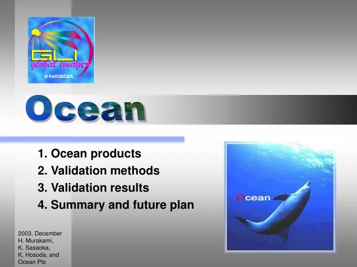
Ocean. 1. Ocean products 2. Validation methods 3. Validation results 4. Summary and future plan. 200 3 , December H. Murakami, K. Sasaoka, K. Hosoda, and Ocean PIs. 1. Ocean products. 200 3 , December H. Murakami, K. Sasaoka, K. Hosoda, and Ocean PIs.

E N D
Ocean 1. Ocean products 2. Validation methods 3. Validation results 4. Summary and future plan 2003, December H. Murakami, K. Sasaoka, K. Hosoda, and Ocean PIs
1. Ocean products 2003, December H. Murakami, K. Sasaoka, K. Hosoda, and Ocean PIs
Overview of GLI ocean products (1) • Ocean atmospheric correction algorithm Developer: Hajime Fikushima (Tokai Univ.) R. Frouin(Scripps institution of oceanography) Algorithm: Atmospheric correction (Fukushima) and Photosynthetically available radiation (Frouin) Algorithm code: OTSK1a (Fukushima), OTSK14 (Frouin) Product code: NL (Level-2) NW/LA (L2Map, L3Bin, L3STAMap) 3 type FR(1km)/LR(4km)/FR_NRT(near real time)for each Parameters: normalized water-leaving radiance (nLw, 13 chs) aerosol radiance (4chs) aerosol optical thickness (Tau), angstrom exp. ocean color quality flag (Bit1-26: quality and cloud info.) photosynthetically available radiation (PAR)(Ein/m2/day)
Overview of GLI ocean products (2) • In-warter algorithms Developer: B.G.Mitchell (Scripps institution of oceanography) Motoaki Kishino(Tokyo University of Marine Science and Technology) Algorithm: In-water algorithms Algorithm code: OTSK2,5,7 (Mitchell), OTSK6 (Kishino) Product code: CS (Level-2) CHLA, CDOM, K490, SS (L2Map, L3Bin, L3STAMap) 3 type FR(1km)/LR(4km)/FR_NRT(near real time)for each Parameters: chlorophyll-a concentration (CHLA), colored dissolved organic matter absorption at 440nm(CDOM) Mitchell attenuation coefficient at490nm(K490), redtide flag, suspended solid concentration (SS),Kishino in-water quality flag(Bit27-32: Case-2 etc.)
Overview of GLI ocean products (3) • Sea surface temperature algorithm Developer: Hiroshi Kawamura (Tohoku Univ.) Algorithm:sea surface temperature Algorithm code:OTSK13 Product code:ST (Level-2, 2Map, 3Bin) ST_daynight, ST_all (L3STAMap) 3 type FR(1km)/LR(4km)/FR_NRT(near real time)for each Parameters: Bulk sea surface temperature (SST) (K), SST quality flag (16bit: cloud information etc.) (cloud detection was improved by EORC and PI)
Near real time operation at direct receiving station GLI ocean operation flow (1/2)(1-km Resolution) L2Map QF_OC L2 Mapping NL_ FR OTSK1a L2Map LA Level 1B H. Fukushima R.Frouin L2Map NW CLFLG CS_FR OTSK2/5/6/7 S. Ackerman K. Stamnes B.G. Mitchell, M. Kishino L2Map CHLA L2Map ST L2Map CDOM L2Map K490 ST_FR OTSK13 L2Map QF_ST L2Map SS H. Kawamura 4-km resampling 16001600 km scene
GLI ocean operation flow (2/2)(4 or 9-km Resolution) 4-km resampling NL_LR OTSK1a L2A_OA CS_LR OTSK2/5/6/7 4-km path ST_LR OTSK13 L3 space bin L3 time bin (Daily, 8-day, Monthly) L3bin NW L3bin LA L3bin CS L3bin ST 9-km equal area grid L3 Statistical Mapping Night ST L3STAMap ST L3STAMap CHLA L3STAMap NW L3STAMap LA L3STAMap CDOM L3STAMap SS L3STAMap K490 9-km global map
Examples of ocean products (1/3)nLw380nm-nLw680 (26 May 2003, California)
CHLA increase Examples (2/3)CHLA, SS, CDOM, K490, Tau, SST… research product: Fluorescence line height
GLI neural network algorithm looks to present CHLA and SS characteristics well. Examples of ocean products (3/3)CHLA and SS distributions SS CHLA
2. Validation methods 2003, December H. Murakami, K. Sasaoka, K. Hosoda, and Ocean PIs
2.3 available match up data Routine observations: GTS (JMA), AERONET, SKYNET, MOBY (MODIS,NOAA) Special observations: 2003.04.03-04.27 California Cooperative Oceanic Fisheries Investigations (CalCOFI) Mitchell (SIO), Frouin (SIO), Hokkaudo Univ. 2003.04-.. Ocean color obs. around Japan Nagasaki Univ., Tokyo Ocean Univ., Nagoya Univ, Tokai Univ., NFRI, Hokkaido Univ, JAMSTEC etc. Relatively many ground observations are provided from PI team and corroborative organizations in the early phase basing relationship until OCTS mission. The data is still increasing, and we continue the data collection and match-up processing now.
2.3 other datasets for evaluation Global distribution can be evaluated by the following datasets. • SeaWiFSglobal dataset (nLw, CHLA, Tau, PAR) • Reynoldsglobal SST data • Tohoku Univ. GMSsolar irradiance dataset (PAR is converted from SW)
3. Validation results 2003, December H. Murakami, K. Sasaoka, K. Hosoda, and Ocean PIs
3.1 vicarious calibration study (1) candidates for the ocean color processing GLI LTOA is compared with simulated LTOA which is calculated using SeaWiFS nLw, pressure, ozone, water vapor, GLI geometry and GLI atmospheric correction look-up tables. We had many data source for the vicarious coefficients. Most of the results show the similar tendencies.
3.1 vical study (2) match-up processing tests • Best choice is SeaWiFS Apr-Jun nLwbase • Possibly temporal change considering SeaWiFS Feb-Mar base coefs. • MOBYcoefs make lower nLw • cannot use Barrowand Railroadones Five Candidates of vical coefs: SeaWiFSApr-Jun/Feb-Mar, Barrow Apr, MOBY 2Fix/Aeronet, Railroad Test data: MOBYand Nagasaki ferry, CalCOFI200304 data number bias CalCOFIobs. are only at CH 4, 6, 9 RMSE ratio
3.2 validation by ground observation match-ups GLI products (nLw) derived using the selected vical coefs show high correlation with ground observations. Figure: nLw380-545 x-axis: ground obs, y-axis: GLIproducts
scattered points are coastal obs. 3.2 validation by match-ups (in-water products) CHLA SS CDOM K490 ground-obs locations
3.2 validation by match-ups (SST) Available data number: 4225 Bias: 0.09K (D:0.06, N:0.17) RMSE: 0.67K(D: 0.67, N: 0.69) 22days sample: 2003/3/19, 3/20, 4/8, 5/28, 6/4, 6/5, 6/10, 6/19, 6/20, 6/30 7/2, 7/5, 7/10, 7/15, 7/19, 7/20, 7/25, 7/30, 8/4, 8/10, 8/19, 9/19
3.3 comparison with other dataset (CHLA) GLI monthly 200304 CHLA distribution agrees with SeaWiFS one SeaWiFS monthly 200304
3.3 comparison with other dataset (PAR) GLI v.s. SeaWiFS PAR GLI monthly 200309 PAR distribution and data range agree well. SeaWiFS monthly 200309
GMS SWPAR 3.3 comparison with other dataset (PAR) GLI v.s. SeaWiFS PAR GLI monthly 200304 GMS monthly 200304 (Kawamura et al., 1998) PAR distribution and data range agree well.
GLI-SST Level-3 STA Map Reynolds-SST GLI SST-Reynolds SST 3.3 comparison with other dataset (SST) AVHRR + buoys(one-degree grid) 4096x2048 (0.088-degree grid) 2003/04/03-22 mean SST • Distribution and data range agree well. • GLI describe fine structure of the ocean current.
4. Summary and future validation plan 2003, December H. Murakami, K. Sasaoka, K. Hosoda, and Ocean PIs
4.1 summary of GLI validationall ocean products can be open today
Ground observations are still needed for the items 4.2 Future validation plan