Download
1 / 19
190 likes | 306 Views
Ensemble Post-Processing and it’s Potential Benefits for the Operational Forecaster Michael Erickson and Brian A. Colle School of Marine and Atmospheric Sciences, Stony Brook University, Stony Brook, NY. High Ensemble Variability: Hanna 9/6/08 00Z Run 18-42 Hour Acc. Precip.

E N D
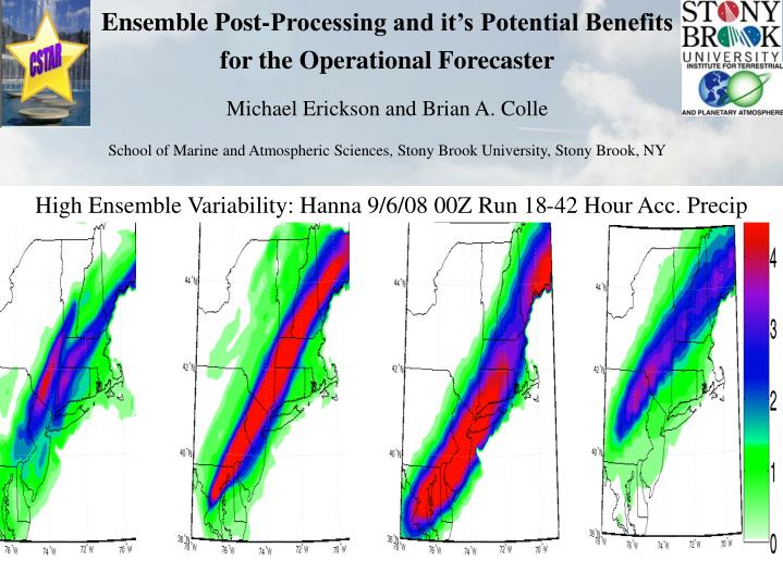
Ensemble Post-Processing and it’s Potential Benefits for the Operational Forecaster Michael Erickson and Brian A. Colle School of Marine and Atmospheric Sciences, Stony Brook University, Stony Brook, NY High Ensemble Variability: Hanna 9/6/08 00Z Run 18-42 Hour Acc. Precip
Ensemble Forecasting Tools: What’s Out There Example from 09 UTC 10/25/2010 – 48 Hr Forecast NCEP SREF Mean 500 hPa Height & Vorticity NCEP SREF 500 hPa 5460 m Contour NCEP SREF Mean SLP and Spread NCEP SREF Low Pressure Positions NCEP SREF Probability of > 35 mph NCEF SREF Probability of > 25 mph NCEP SREF Probability of > 25 mph NCEP SREF Probability > 1” Precipitation NCEP SREF Mean 12-hr Snow Sources: http://www.spc.noaa.govexper/sref & http://www.meteo.psu.edu/~gadomski/ewallsref.html/
Motivation NCEP SREF Temperature Bias > 24oC 2X Bias • Ensembles have biases which can affect both the ensemble mean and probabilistic results. • Can post-processing model data improve both the biases and probabilities derived from the ensemble? No Bias Goals • Evaluate the deterministic and probabilistic biases within the Stony Brook University (SBU) and Short Range Ensemble Forecast (SREF) ensembles. • Apply bias correction and a post-processing technique known as Bayesian Model Averaging (BMA) to the ensembles. • Show how post-processing can be used by operational forecasters and its potential application to river flood forecasting.
Methods and Data Accumulated Stage IV Rain Data Verification Domain Region of Study • Analyzed the 00 UTC 13-member Stony Brook University (SBU) and the 21 UTC 21-member Short Range Ensemble Forecast (SREF) system run at NCEP for temperature and precipitation. • Observations consist of the Automated Surface Observing System (ASOS) for temperature and Stage IV rain data for precipitation. • Stage IV data is a blend of rain gauge observations and radar derived rain estimates. • Results are for the 2007-2009 warm seasons (4/1-9/31).
The SBU/SREF Ensemble SBU 13 Member Ensemble NCEP SREF 21 Member Ensemble Region of Study • 7 MM5 and 6 WRF members run at 12-km grid spacing nested within a 36-km domain. • Ensemble uses a variety of initial conditions (GFS, NAM, NOGAPS,and CMC), two cloud microphysical, three convective, and three planetary boundary layer schemes. • 10 ETA members at 32 km grid spacing. • 5 RSM members at 45 km grid spacing. • 3 WRF-NMM members at 40 km grid spacing. • 3 WRF-ARW members at 45 km grid spacing. • IC's are perturbed using a breeding technique. Verification Domain 12-km Model Domain
Model Biases 2007-2009 - Temperature Raw Bias > 24oC for MYJ WRF Member Model Bias by Member > 24oC Diurnal Mean Error
Bias Correction: Cumulative Distribution Function (Hamill and Whitaker 2006) • A 50-day training period was used to calculate the cumulative distribution function (CDF) of each model and the observation. • The model CDF was then adjusted to the observation over the calibration and validation period value by value. • To correct for spatial bias associated with terrain, the bias for each elevation was calculated and removed using a binning approach. CDF Bias Correction Example CDF For Model and Observation
Bias Correction 2007-2009 - Temperature Raw Bias > 24oC for MYJ WRF Member Diurnal Root Mean Squared Error Model Bias by Member > 24oC Bias Corrected > 24oC for MYJ WRF Member Bias Corrected Diurnal RMSE Diurnal Mean Error
Model Biases 2007-2009 - Precipitation Raw Bias > 0.5” for MYJ WRF Member Model Bias by Member > 0.1” Model Bias by Member > 1”
Bias Correction 2007-2009 - Precipitation Model Bias by Member > 0.1” Bias Corrected > 0.5” for MYJ WRF Member Model Bias by Member > 1”
Ensemble Underdispersion and Reliability Reliability for Precip > 0.5” Reliability for Temp > 24oC Temp Rank Histogram Precip Rank Histogram • Although biases have been largely corrected, the ensemble is still underdispersed and has unreliable probabilistic forecasts. • Additional post-processing is necessary so that more accurate probabilistic forecasts can be obtained.
Bayesian Model Averaging (BMA) • Bayesian Model Averaging (BMA, Raftery et al. 2005) is designed to improve ensemble forecasts by estimating two things: • The weights for each ensemble member (i.e. a “better” member will have more influence on the forecast. • The uncertainty associated with each forecast (i.e. a forecast should not be thought of as a point, but as a distribution). • Although BMA has been shown to improve ensemble mean forecasts, its main advantage is with probabilistic forecasts. The BMA derived distribution The coldest member is given the greatest weight The warmer members have varying weights The second coldest member is given significantly less weight From Raftery et al. 2005
BMA Weights – 2007-2009 Precipitation SBU Member Weights SREF Member Weights
Impact of BMA on Reliability after Bias Correction for Warm Season Surface Temperature (2007-2009) Bias Corrected Rank Histogram Reliability > 20oC BMA Rank Histogram Brier Skill Scores BMA Corrected Bias Corrected -5 0 5 10 15 20 (C)
Impact of BMA on Reliability after Bias Correction for Warm Season Surface Temperature (2007-2009) Bias Corrected Rank Histogram Reliability > 0.5” BMA Rank Histogram Brier Skill Scores BMA Corrected Bias Corrected
12 – 36 Hr Accumulated Precipitation Raw Ensemble Probability > 1.5” Bias Cor. Ensemble Probability > 1.5” BMA Ensemble Probability > 1.5” BMA Ensemble Probability > 1.5” Stage IV Rain Data Post-Processing Application - 5/17/10 21z NCEP SREF
6 – 36 hr Accumulated Precipitation Raw Ensemble Probability > 1.5” Bias Cor. Ensemble Probability > 1.5” BMA Ensemble Probability > 1.5” Stage IV Rain Data Hanna - 9/5/08 21z NCEP SREF
Tropical Hanna Case: Hydrological Test Case 9/6/08 00z Run: Saddle River: Lodi, NJ QPF from Ensemble Modeled Response: NWS River Forecast System 12 cm 9 cm 6 cm 3 cm 0 cm Observed Flood Stage ~2.3 m 3.5m 3.0m 2.5m 2.0m 1.5m 1.0m -33% of members predict major flooding -42% of members predict moderate flooding -58% of members predict flooding • Future work will investigate the potential benefits of BMA for streamflow and flood risk assessment.
Conclusions • Ensemble members suffer from large biases for surface parameters, which can vary temporally, spatially, diurnally and between members. • The bias correction and BMA improves the probabilistic skill, reliability and dispersion of the Stony Brook + NCEP SREF ensemble. • Since post-processing improves the ensemble performance spatially, forecasters/users could use BMA for gridded forecast products. • Although post-processing can remove some systematic biases, it can not correct fundamental problems within the model. For instance, BMA can not correct for large position errors in precipitation forecasts. • Further development with BMA is needed for extreme weather events such as high QPF forecasts and river flood forecasts given the smaller sample size.