Download
1 / 37
390 likes | 476 Views
Dive into the world of chemical thermodynamics with a bond-graphic interpretation, understanding mass and heat flows in chemical reactions, and exploring causality in bond graphs. Learn about conversions, stoichiometry, periodic table elements, equation of state, Gibbs equation, and chemical reactor models.

E N D
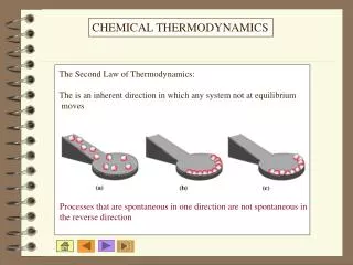
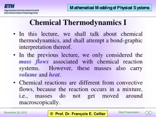
In this lecture, we shall talk about chemical thermodynamics, and shall attempt a bond-graphic interpretation thereof. In the previous lecture, we only considered the mass flows associated with chemical reaction systems. However, these masses also carry volume and heat. Chemical reactions are different from convective flows, because the reaction occurs in a mixture, i.e., masses do not get moved around macroscopically. Chemical Thermodynamics I
Yet, some reactions change the overall volume (or pressure) of the reactants, such as in explosive materials, others occur either exothermically or endothermically. It is obviously necessary to keep track of these changes. Furthermore, we chose to represent substances in a mixture by separate CF-elements. If we wish to continue with this approach, volume and heat flows indeed do occur between these capacitive fields. Chemical Thermodynamics II
Causality in chemical bond graphs Conversion between mass and molar flow rates Stoichiometry Periodic table of elements Equation of state Isothermal and isobaric reactions Gibbs equation Chemical reactor model Table of Contents I
Mass balance Energy balance Volume flow Entropy flow Improved chemical reactor model Multi-bus-bonds Chemical multi-port transformers Chemical resistive fields Table of Contents II
mix reac MTF CF RF N mix reac Since the N-matrix cannot be inverted, the causality of the chemical MTF-element is fixed. The CF-element computes the three potentials (T, p, g), whereas the RF-element computes the three flows (S, q, M) of each substance involved in the reaction. · · Causality in Chemical Bond Graphs • Let us look once more at the generic chemical reaction bond graph:
m g TF · n M m Conversion Between Mass Flow Rateand Molar Flow Rate • The molar flow rate is proportional to the mass flow rate. Thus, we are dealing here with a regular transformer. • The transformation constant, m, depends on the substance. For example, since 1 kg of H2 correspond to 500 moles, mH2 = 0.002. • The entropy flow and heat flow don’t change.
} State information needs to be copied over by equations. The TFch-Element • Hence it makes sense to create the following chemical transformation element:
As we saw in the previous lecture, the generic chemical reaction bond graph can be decomposed into a detailed bond graph showing individual flows between reactants and reactions. In such a bond graph, the stoichiometric coefficients are represented by transformers. However, since the mass flow rate truly changes in such a transformer (this is not merely a conversion of units), the entropy and heat flows must change along with it. Stoichiometric Coefficients
The TFst-Element • Hence it makes sense to create the following stoichiometric transformation element:
We can consult the periodic table of elements: 1 mole = 80 g Periodic Table of Elements
Stoichiometry · CS ChR mk1 = –mBr2 + 2mBr· · 2n · · 2m Br · · · · m m g n k1 · k1 M Br M CS 1 mole = 160 g 1 mole = 80 g Br Br Br Br Br Br2 Br2 n n n m m m n g k1 k1 k1 k1 Br2 Br2 Br2 Br2 Br2 = –k1 + k2 – k5 k1 Br2 2Br·
Chemical substances satisfy a so-called equation of state that relates the three domains to each other. For ideal gases, the equation of state can be written as follows: The equation of state can be written either for partial pressures (Dalton’s law) or for partial volumes (Avogadro’s law). R = 8.314 J K-1 mole-1 is the gas constant pi · V = ni· R · T p · Vi = ni· R · T Dalton’s law Avogadro’s law The Equation of State p · V = n · R · T
If both pressure and temperature can be assumed approximately constant, the equation of state can be conveniently differentiated as follows (using Avogadro’s law): p · qi = ni· R · T This equation can be used to compute the volume flow from the mass flow: R · T p qi = ni· Isothermal and Isobaric Reactions I p · Vi = ni· R · T
This relationship holds for all flows in the hydrogen-bromine reaction, thus: pk1 –1 +20 0 0 pBr2 pk2+1–2 000pBr· pk3 = 0 –1–1+1+1·pH2 pk40 +1 +1–1–1 pH· pk5-1 +1 0–1+1 pHBr describe the corresponding partial pressures. Isothermal and Isobaric Reactions II qBr2 –1 +10 0 -1 qk1 qBr· +2 –2 –1+1+1 qk2 qH2 = 0 0 –1+10 ·qk3 qH· 0 0 +1–1–1 qk4 qHBr 0 0 +1–1+1 qk5
Chemical substances also satisfy the so-called Gibbsequation, which can be written as: Since we already know ni and qi, we can use this equation to compute Si. The entropy flow accompanies the mass flow and the volume flow. Due to linearity (T, p = constant m = constant), the entropy flow can be superposed to the mass and volume flows. · p · qi = T · Si + m · ni The Gibbs Equation ·
Entropy flows for the hydrogen-bromine reaction: SBr2 –1 +10 0 -1 Sk1 SBr· +2 –2 –1+1+1 Sk2 SH2 = 0 0 –1+10 ·Sk3 SH· 0 0 +1–1–1 Sk4 SHBr 0 0 +1–1+1 Sk5 Isothermal and Isobaric Reactions III Neither the partial entropies nor the (physically extremely dubious!) “partial temperatures” are used anywhere, except for defining the corresponding power flows. · · · · · · · · Tk1 –1 +20 0 0 TBr2 · · Tk2+1–2 000TBr· Tk3 = 0 –1–1+1+1·TH2 Tk40 +1 +1–1–1 TH· Tk5-1 +1 0–1+1 THBr describe the corresponding “partial temperatures.”
· · CS CS ChR ChR · 2n 2q · · · 2m 2p Br Br · · · · · · · m n p m p q g k1 k1 · k1 k1 M Br Br M CS CS Br Br Br Br Br Br Br Br Br2 Br2 Br2 q q n n p n q m q p n m m g p k1 k1 k1 k1 k1 k1 k1 k1 Br2 Br2 Br2 Br2 Br2 Br2 Br2 k1 Br2 2Br·
· · CS CS ChR ChR · · 2S 2n · · · 2T 2m Br Br · · · · · · · T m n T S m g k1 k1 · k1 k1 M Br Br M CS CS Br Br Br Br Br Br Br Br Br2 · Br2 Br2 S S S T m n n n S m m g T T n k1 k1 k1 k1 k1 k1 k1 k1 Br2 Br2 Br2 Br2 Br2 Br2 Br2 · · · · k1 Br2 2Br·
We are now ready to sketch the combined model: This model is still to be discussed. It requires state information from all reactants. · CF ChR Br k1 CF This is now the standard capacitive field, as it had been introduced in the discussion of the convective flows. Br2 The Bus-1-Junction does not propagate the state information. k1 Br2 2Br·
We already know that the chemical reactor needs to compute the three flows. We already have the equations for this model: nk1 = k1· nBr2 qk1 = nk1· (R · T)/p Sk1 = (p · qk1 - mk1 ·nk1 )/T reaction rate equation equation of state · Gibbs equation The Chemical Reactor Model I We still need to verify though that no balance equations are being violated!
The mass balance is embedded in the stoichiometric coefficients. Whatever gets removed from one reactant, gets added back to another. Hence the total reaction mass will not change. This is true for each step reaction separately, since each step reaction must satisfy the stoichiometric constraints. Mass Balance
The way the equations were set up, we already know that: and due to the symmetry of the other two domains: Hence the change in internal energy can be written as: · · Tmix’· Smix= Treac’· Sreac · · U = Tmix’· Smix-pmix’· qmix+ mmix’· nmix · = Treac’· Sreac-preac’· qreac+ mreac’· nreac Energy Balance I mmix’· nmix= mreac’· nreac pmix’· qmix= preac’· qreac
The above equation holds true under all operating conditions, i.e., the topology of the chemical reaction network is independent of the conditions under which the chemical reaction is performed. The isothermal and isobaric conditions assumed before only influence the CF-field, i.e., the way in which the three potentials are being computed, and possibly the RF-field, i.e., the way in which the three flows are being computed (we shall discuss in the next class, whether this is indeed true or not). Energy Balance II
Under isothermal and isobaric conditions, we can write: qk1 = nk1· (R · T)/p qk2 = nk2· (R · T)/p qk3 = nk3· (R · T)/p qk4 = nk4· (R · T)/p qk5 = nk5· (R · T)/p pk1 –1 +20 0 0 pBr2 +1 pk2+1–2 000pBr· –1 pk3 = 0 –1–1+1+1·pH2 = 0 · p pk40 +1 +1–1–1 pH· 0 pk5-1 +1 0–1+1 pHBr 0 preac’· qreac = (nk1 – nk2 ) · (R · T) = pmix’· qmix Volume Flow I
However under isobaric conditions, we can also write: pmix’· qmix = p· ones(1,5) · qmix = p· ones(1,5) · nmix · (R · T)/p = ones(1,5) · nmix · (R · T) = ones(1,5) · N · nreac · (R · T) = (nk1 – nk2 ) · (R · T) = preac’· qreac Volume Flow II
Let us now discuss the entropy flow. We are certainly allowed to apply the Gibbs equation to the substances: Under isothermal and isobaric conditions: Thus: · Tmix’· Smix= pmix’· qmix- mmix’· nmix · T· ones(1,5) · Smix= p· ones(1,5) · qmix- mmix’· nmix Entropy Flow I · T· ones(1,5) · N · Sreac= p· ones(1,5) · N · qreac- mreac’· nreac
Therefore: Thus, the Gibbs equation can also be applied to reactions. · · T· (Sk1 – Sk2 )= p· (qk1 – qk2)- mreac’· nreac · Sk1 = (p· qk1 - mk1· nk1)/T · Sk2 = (p· qk2 - mk2· nk2)/T · Sk3 = (p· qk3 - mk3· nk3)/T · Sk4 = (p· qk4 - mk4· nk4)/T · Sk5 = (p· qk5 - mk5· nk5)/T Treac’· Sreac = T· (Sk1 – Sk2 ) = Tmix’· Smix · · · · Entropy Flow II Tk1 –1 +20 0 0 TBr2 +1 Tk2+1–2 000TBr· -1 Tk3 = 0 –1–1+1+1·TH2 = 0 · T Tk40 +1 +1–1–1 TH· 0 Tk5-1 +1 0–1+1 THBr 0
We are now ready to program the chemical reactor model. nk1 = k1· nBr2 qk1 = nk1· (R · T)/p Sk1 = (p · qk1 -mk1 ·nk1 )/T · The Chemical Reactor Model II
Consequently: · CF Br CF Br2 Effort sensor State sensor The Chemical Reactor Model III The activated bonds are awkward. They were necessary because stuff got separated into different and no longer neighboring models that are in reality different aspects of the same physical phenomenon.
A clean solution is to create a new bond graph library, the ChemBondLib, which operates on multi-bus-bonds, i.e. vectors of bus-bonds that group all of the flows together. Special “blue” multi-bus-0-junctions will be needed that have on the one side a group of red bus-bond connectors, on the other side one blue multi-bus-bond connector. The individual CF-elements can be connected to the red side, whereas the MTF-element is connected to the blue side. The Multi-Bus-Bond
The MTF-element is specific to each reaction, since it contains the N-matrix, which is used six times inside the MTF-element: nreac = N · nmix qreac = N · qmix Sreac = N · Smix mmix = N’ · mreac pmix = N’ · preac Tmix = N’ · Treac · · The MTF-Element
The RF-element is also specific to each reaction, and it may furthermore be specific to the operating conditions, e.g. isobaric and isothermal. In the isobaric and isothermal case, it could contain the vector equations: The RF-Element n = [ nBr2 ; nBr· 2/V ; nH2*nBr· /V ; nHBr * nH· /V ; nH· * nBr2 /V ] ; nreac = k .* n ; p * qreac = nreac * R * T ; p * qreac = T * Sreac + mreac .* nreac ; ·
In my Continuous System Modelingbook, I had concentrated on the modeling the reaction rates, i.e., on the mass flow equations. I treated the volume and heat flows as global properties, disassociating them from the individual flows. In this new presentation, I recognized that mass flows cannot occur without simultaneous volume and heat flows, which led to an improved and thermodynamically more appealing treatment. Conclusions I
Although I had already recognized in my book the N-matrix, relating reaction flow rates and substance flow rates to each other, and although I had seen already then that the relationship between the substance chemical potentials and the reaction chemical potentials was the transposed matrix, M = N’, I had not yet recognized the chemical reaction network as a bond-graphic Multi-port Transformer (the MTF-element). Although I had recognized the CS-element as a capacitive storage element, I had not recognized the ChR-element as a reactive element. Conclusions II
When I wrote my modeling book, I started out with the known reaction rate equations and tried to come up with a consistent bond-graphic interpretation thereof. I took the known equations, and fit them into boxes, wherever they fit best … and in all honesty, I didn’t goof up very much doing so, because there aren’t many ways, using the bond-graphic technique, that would lead to a complete and consistent (i.e., contradiction-free) set of equations, and yet be incorrect. Conclusions III
However, the bond-graphic approach to modeling physical systems is much more powerful than that. In this lecture, I showed you how this approach can lead to a clean and consistent thermo-dynamically appealing description of chemical reaction systems. We shall continue with this approach during one more class, where I shall teach you a yet improved way of looking at these equations. Conclusions IV
Cellier, F.E. (1991), Continuous System Modeling, Springer-Verlag, New York, Chapter 9. Cellier, F.E. and J. Greifeneder (2009), “Modeling Chemical Reactions in Modelica By Use of Chemo-bonds,” Proc. 7th International Modelica Conference, Como, Italy, pp. 142-150. References